HyperBloch#

In this tutorial we will see how the cell, model and supercell model graphs, constructed through HyperCells, can be imported and visualized in the Poincaré disk through the HyperBloch package. Moreover, we go through the intended workflow for the construction of corresponding Abelian Bloch Hamiltonians in order to demonstrate the supercell method through density of states calculations.

Prerequisits in GAP#

In order to get started with the HyperBloch package we construct nearest-neighbor graphs of the {8,8}-tessellation of the hyperbolic plane through the HyperCells package in GAP. We first construct the primitive cell and the model graph (based on the tessellation graph), and finally the supercell, as we have established previously in getting started with HyperCells package:

# load the HyperCells package
LoadPackage( "HyperCells" );

# set up (proper) triangle group
tg := ProperTriangleGroup( [ 2, 8, 8 ] );

# Primitive cell:
# ---------------

# specify the quotient defining the primitive cell
qpc := TGQuotient( [ 2, 6 ] );

# construct symmetric primitive cell
cgpc := TGCellGraph( tg, qpc, 3 : simplify := 5 );
Export( cgpc, "(2,8,8)_T2.6_3.hcc" ); # export

# elementary nearest-neighbor model
model := TessellationModelGraph( cgpc, true : simplify := 0 );
Export( model, "{8,8}-tess_T2.6_3.hcm" ); # export

# Supercell:
# ----------

# specify the quotient defining the supercell cell
qsc := TGQuotient( [ 3, 11 ] );

# construct symmetric supercell
cgsc := TGCellGraph( tg, qsc, 3 : simplify := 3 );
Export(cgsc, "(2,8,8)_T3.11_3.hcc");

# construct symmetric supercell
sc := TGCellSymmetric( tg, qsc, 3 );

# extend the model defined on the primitive cell to the supercell
scmodel := TGSuperCellModelGraph( model, sc : simplify := 0);
Export( scmodel, "{8,8}-tess_T2.6_3_sc-T3.11.hcs" ); # export

Download generated files Download GAP Code

Hands-on in Mathematica#

Next, in Mathematica, we load the HyperBloch package and set the current directory to the working directory, assuming it contains the HyperCells files created above:

<< PatrickMLenggenhager`HyperBloch`
SetDirectory[NotebookDirectory[]];

Primitive cell#

Import the cell graph#

The cell graph defines a maximally symmetric triangular tessellation of the corresponding connected and compactified translation unit cell. We import it with the function ImportCellGraphString:

pcell = ImportCellGraphString[Import["(2,8,8)_T2.6_3.hcc"]];

Note the use of the Import function inside the ImportCellGraphString function. This is necessary, because the exported file is a text file, which contains the string representation of the cell graph. The Import function is used to read the file, while the ImportCellGraphString function is used to parse the string and construct the cell graph. Alternatively, we could have used the function ExportString in GAP to export the cell graph as a string, copied the string into a Mathematica notebook, and then used the ImportCellGraphString function (or one of the analogous functions) directly to parse the string and construct the cell graph.

Import the model graph#

The model graph is derived from cell graph. In our case it defines a nearest-neighbor graph of the \(\{8,8\}\)-tesselation of the hyperbolic plane restricted to the primitive cell. It can be imported analogously, but requires the use of the function ImportModelGraphString in order to parse the string and construct the model graph instead:

pcmodel = ImportModelGraphString[Import["{8,8}-tess_T2.6_3.hcm"]];

Visualize the the model graph#

The HyperBloch package provides convenient functions for the visualization of graph representations of models on unit cells. We can visualize the model graph with the function VisualizeModelGraph:

VisualizeModelGraph[pcmodel,
  CellGraph -> pcell,
	Elements -> <|
		ShowCellBoundary -> {ShowEdgeIdentification -> True},
		ShowCellGraphFlattened -> {}
	|>,
  ImageSize -> 300,
  NumberOfGenerations -> 2]

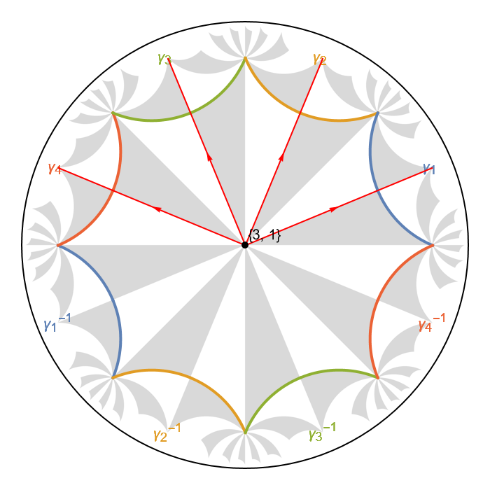
producing a figure of an elementary nearest-neighbor model on the \(\{8,8\}\)-lattice:

The function ShowCellGraphFlattened is used to shown all edges connecting pairs of vertices as hyperbolic geodesics in the Poincaré disk. We have passed the cell graph to the option CellGraph which enables us to indicate the unit cell boundary through the function ShowCellBoundary. Moreover, the boundary segments are indicated together with the associated (composite) translations in the translation group \(\Gamma_{pc}\) and colored according to the boundary identification.

We can further emphasize the Schwarz triangles inside the indicated primitive cell through the function ShowCellSchwarzTriangles:

VisualizeModelGraph[pcmodel,
  CellGraph -> pcell,
  Elements -> <|
   	ShowCellBoundary -> {ShowEdgeIdentification -> True},
   	ShowCellSchwarzTriangles -> {TriangleStyle -> FaceForm[GrayLevel[0.5]]}
  |>,
  ImageSize -> 300,
  NumberOfGenerations -> 2]

There are 8 Schwarz triangles in the primitive cell associated with the chosen representatives in the right transversal \(T_{\Delta^{+}}(\Gamma_{pc})\).

Construct the Hamiltonian#

In order to construct the Abelian Bloch Hamiltonian, parameters need to be assigned to the vertices and the edges in the model graph. This takes a very compact form for an elementary nearest-neighbour tight-binding model. In order to illustrate the procedure, we will start with the most general assignment strategy and demonstrate the compact form afterwards.

Skip to subsection Compact strategy

On a first reading, you may want to skip the section “General strategy” and continue with the section “Compact strategy”.

General strategy#

Number of orbitals#

Every model graph can be equipped with multiple orbitals per site, and even with a varying number of orbitals at each site. We will construct more involved models with multiple orbitals per site in the Higher-order topology tutorial, for now, however, we will set the number of orbitals to one:

norbits = 1;

Next, we need to assign the parameters which describe the tight-binding model. This is achieved through the vertices and edges specified in the model graph. Each, should be associated with a coupling constant such that they can be called through a function or an Association.

On-site terms#

On-site terms in the Hamiltonian are associated with vertices in the model graph. As such, it is instructive to explicitly print these vertices by using the function VertexList, which takes as argument the graph representation:

VertexList@pcmodel["Graph"]

There is only one site residing in this particular primitive cell of the \(\{8,8\}\)-lattice, as such the vertex list contains only one entry {{3, 1}}. Each vertex is given in the form {w, gi}, where w is an integer between 1 and 3 indicating the type of vertex of the Schwarz triangle (x, y, z), i.e., a Wyckoff position, and gi is the position in the transversal \(T_{G^+}(G_{w}^{+})\) labeling the Schwarz triangle the vertex is a part of, as specified in any HCModelGraph.

We choose to set the on-site term to zero by associating the list of vertices with a list of zeros using an Association:

mVec = ConstantArray[0, 1]; 
onsitePC = AssociationThread[VertexList@pcmodel["Graph"] -> mVec];

Hopping terms#

The hopping terms are associated with edges in the model graph. In analogy with the on-site terms, it is useful to explicitly print the edges using the function EdgeList, which takes as argument the graph representation:

EdgeList@pcmodel["Graph"]

Each element in the list is a DirectedEdge, connecting a pair of vertices. The EdgeTags (nested list above the arrows) for the nearest-neighbour edges take the form {1, {ve, s1, s2}}, where the first entry, 1, indicates a nearest-neighbor edge, ve={w, g} specifies the cell-graph edge vertex with w the type of vertex and g the position of the element in \(T_{G^{+}}(G_{w}^{+})\), and s1, s2 are the positions of the Schwarz triangles associated with the cell-graph edges in \(T_{\Delta^{+}}(\Gamma)\). However, this labeling convention comes with some exceptions, which we will explore in more the more involved HyperBloch package tutorials.

We choose to set the hopping terms to a constant real value \(-1\) for all edges by associating the edge list with a list of constant values:

nnHoppingVec = ConstantArray[-1, 4];
hoppingPC = AssociationThread[EdgeList@pcmodel["Graph"] -> nnHoppingVec];

If we would consider a more involved model it might be helpful to look at the translation operators associated with the edges:

pcmodel["EdgeTranslations"]

which contains the translation operators {g1, g4, ... }. In our particular case, all edges are associated with a non-trivial translation, i.e., the parameters we have assigned are inter-cell hopping amplitudes.

The HyperBloch package is equipped with elaborate visualization tools of cell, model and supercell model graphs which can further guide the construction of models in more advanced settings. We will exploit these in subsequent tutorials.

Hamiltonian#

The Abelian Bloch Hamiltonian can now be set up by passing the model graph and the corresponding coupling constants specified above as arguments to the function AbelianBlochHamiltonian or alternatively AbelianBlochHamiltonianExpression, the former returns the Hamiltonian as a function of momenta. We choose to use the latter for now, in order to print a symbolic expression of the Hamiltonian:

Hpc = AbelianBlochHamiltonianExpression[pcmodel, norbits, onsitePC, hoppingPC]

which in this particular example constructs a \(1\times1\) matrix as a function of four momenta:

{ { -2 (Cos[k[1]] + Cos[k[2]] + Cos[k[3]] + Cos[k[4]]) } }

Compact strategy#

The simplicity of the specified model reduces the construction of the Hamiltonian to just one line of code. Once again we set the number of orbitals per site in the second argument to \(1\), the on-site term to \(0\) and the nearest-neighbor coupling to \(-1\), with the function AbelianBlochHamiltonian, which returns the Hamiltonian as a function of momenta. A very economic way to do this is through the use of constant Functions instead of Associations:

Hpc = AbelianBlochHamiltonian[pcmodel, 1, 0 &, -1 &];

For more efficient evaluation, we precompile the Bloch Hamiltonian by specifying the option CompileFunction->True:

Hpccf = AbelianBlochHamiltonian[pcmodel, 1, 0 &, -1 &, CompileFunction -> True];

Density of states#

To compute the density of states, we can now take advantage of the independence of different momentum sectors and therefore parallelize the computation of the eigenvalues. We take a set of Npts random samples in momentum space and partition this set into Nruns subsets. The dimension of Brillouin zone is defined by the genus of the compactified primitive cell and is \(2 \cdot genus\), which we specify by passing the genus as an argument. As such, we compute the eigenvalues with the following function:

ComputeEigenvalues[cfH_, Npts_, Nruns_, genus_] := 
  Flatten @ ParallelTable[
    Flatten @ Table[
      Eigenvalues[cfH @@ RandomReal[{-Pi, Pi}, 2 genus]], 
    {i, 1, Round[Npts/Nruns]}], {j, 1, Nruns}, 
  Method -> "FinestGrained"]

We compute the eigenvalues with a set of \(10^6\) random samples in momentum space and \(32\) subsets:

evspc = ComputeEigenvalues[Hpc, 10^6, 32];

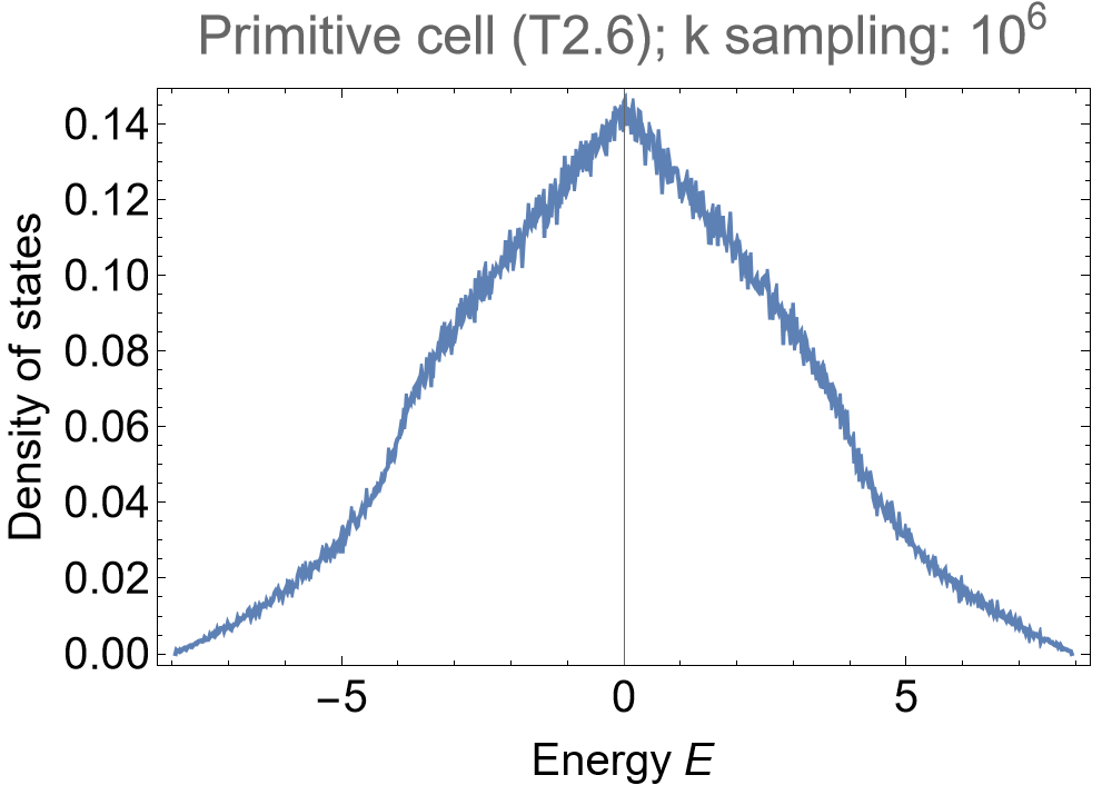
We choose to visualize the density of states via a kernel density estimation with an energy binwidth of \(0.005\) for the elementary nearest-neighbor model on the primitive cell of the \(\{8,8\}\)-lattice:

SmoothHistogram[evals, 0.005, "PDF",
  Frame -> True, FrameLabel -> {"Energy E", "Density of states"} FrameStyle -> Black, 
  ImageSize -> 500, ImagePadding -> {{Automatic, 10}, {Automatic, 10}}, LabelStyle -> 20,
  PlotLabel -> "Primitive cell (T2.6); k sampling: 10^6", PlotRange -> All]

density of Abelian Bloch states of the elementary nearest-neighbor model on the primitive cell T2.6 of the {8,8} lattice

First supercell#

Import the cell and supercell model graph#

The cell graph for the compactified translation supercell can be imported like the one for the primitive cell through the function ImportCellGraphString:

scell = ImportCellGraphString[Import["(2,8,8)_T3.11_3.hcc"]];

The supercell model graph is derived from cell graph can be imported analogously, but requires the use of the function ImportSupercellModelGraphString instead:

scmodel = ImportSupercellModelGraphString[Import["{8,8}-tess_T2.6_3_sc-T3.11.hcs"]];

Visualize the supercell model graph#

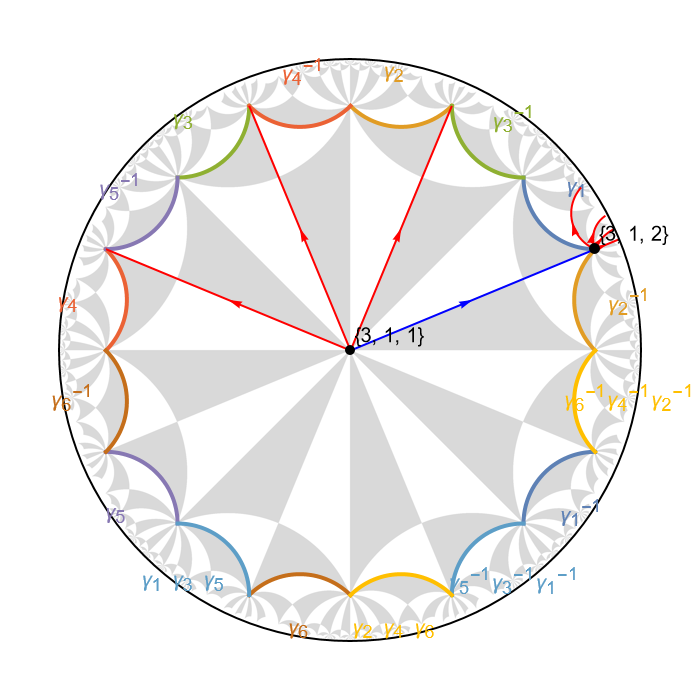
Let us visualize the supercell model representation of the nearest-neighbor model:

VisualizeModelGraph[scmodel,
  CellGraph -> scell,
  Elements -> <|
    ShowCellBoundary -> {ShowEdgeIdentification -> True},
    ShowCellGraphFlattened -> {}
  |>,
  ImageMargins -> 0, ImagePadding -> 15, 
  ImageSize -> 300, NumberOfGenerations -> 3]

Let us further emphasize the Schwarz triangles inside the indicated supercell:

VisualizeModelGraph[scmodel,
  CellGraph -> scell,
  Elements -> <|
    ShowCellBoundary -> {ShowEdgeIdentification -> True},
    ShowCellSchwarzTriangles -> {
      TriangleStyle -> Directive[ Opacity[0.6], FaceForm[GrayLevel[0.5]]]
      }
  |>,
  ImageSize -> 300, ImageMargins -> 0,
  ImagePadding -> 15, NumberOfGenerations -> 3]

There are 16 Schwarz triangles in the supercell associated with the chosen representatives in the right transversal \(T_{\Delta^{+}}(\Gamma_{sc})\), as such this particular supercell consists of a symmetric aggregation of two primitive cells.

Since the model on the primitive cell already defines all the necessary model specification for the supercell, we do in general not need to explicitly print the vertices and edges of supercell model graphs. However, it is instructive to do so in order to understand the underlying mechanism:

Skip to subsubsection Hamiltonian and density of states

On a first read one may want to skip the next two subsubsection “Vertices” and “Edges” and continue at the subsection “Hamiltonian and density of states”.

Vertices#

Analogous to the model graph, the vertices can be extracted by using the function VertexList, which takes as argument the graph representation:

VertexList@scmodel["Graph"]

There are two site residing in this particular supercell {{3, 1, 1}, {3, 1, 2}}. Vertices in the supercell model graphs are given in the form {w, gi, etaj}, where w is an integer between 1 and 3 indicating the type of vertex of the Schwarz triangle (x, y, z), gi is the position in the transversal \(T_{G^{+}}(G_{w}^{+})\) labeling the Schwarz triangle the vertex is a part of, and etaj the position of the element in the transversal \(T_{\Gamma_{pc}}(\Gamma_{sc})\) labeling the copy of the primitive cell containing the vertex inside the supercell, as specified in any HCSupercellModelGraph.

Edges#

Similarly, the edges can be extracted by using the function EdgeList, which takes as argument the graph representation:

EdgeList@scmodel["Graph"]

The edge tags are of the form {v1pc, v2pc, tagpc} with v1pc, v2pc the positions of the vertices in the primitive cell, and tagpc the tag of the edge in the primitive cell. However, also this labeling convention comes with some exceptions, which we will explore in more the more involved HyperBloch package tutorials.

Hamiltonian and density of states#

The construction of the model on the primitive cell already defines all the necessary model specification for the supercell. In order to construct the elementary nearest-neighbor tight-binding model on the supercell, we just need to replace the model graph with the supercell model graph in the first argument in the function AbelianBlochHamiltonian. In addition, we also need to specify the associated model graph with the option PCModel. This already captures some of the higher-dimensional irreducible representations on the original primitive cell:

Hsccf = AbelianBlochHamiltonian[scmodel, 1, 0 &, -1 &, PCModel -> pcmodel, CompileFunction -> True];

We compute the Eigenvalues with a set of \(10^5\) random samples in momentum space and \(32\) subsets:

evssc = ComputeEigenvalues[Hsc, 2*10^5, 32];

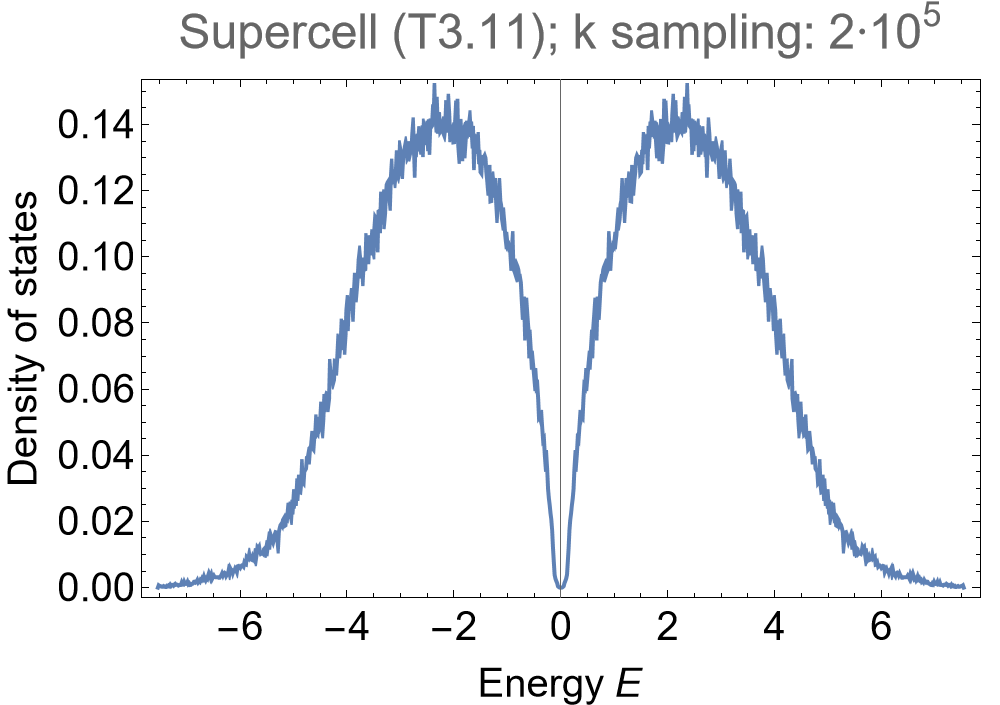
Once again, we choose to visualize the density of states via a kernel density estimation with an energy binwidth of \(0.005\) for first consecutive supercell of the primitive cell:

SmoothHistogram[evssc, 0.005, "PDF",
  Frame -> True, FrameLabel -> {"Energy E", "Density of states"} FrameStyle -> Black, 
  ImageSize -> 500, ImagePadding -> {{Automatic, 10}, {Automatic, 10}}, LabelStyle -> 20,
  PlotLabel -> "Primitive cell (T2.6); k sampling: 2*10^5", PlotRange -> All]

density of states of the elementary nearest-neighbor model on the {8,8} lattice as computed using the supercell method with sequence T2.6, T3.11, T5.13, T9.20, T17.29, T33.44, T65.78

Download Mathematica Notebook

Aspects of the content above originate from the Supplementary Data and Code, where more examples are provided and the necessary steps to find the density of states of an elementary nearest-neighbor hopping model on the \(\{8,8\}\)-lattice are discussed in detail.