Higher-order topology#
Learning goals
Construction of:
elementary nearest-neighbor model with multiple orbitals per site,
finite flakes and the computation of energy spectra with open boundary conditions
and construction of disclination defects with negative Frank angles.
Featured functions
HyperBloch:
AbelianBlochHamiltonian, IntroduceDisclination, ShowCellBoundary, ShowCellGraphFlattened, TBHamiltonian, VisualizeModelGraph
Needed functions
Mathematica:
In previous tutorials, such as Getting started with the HyperBloch package and HyperBloch Supercells tutorial etc., we have calculated the density of states of various nearest-neighbor tight-binding models via exact diagonalization and random samples. We predefine a function in order to calculate the eigenvalues for the Abelian Bloch Hamiltonians that we will construct. We take advantage of the independence of different momentum sectors and parallelize the computation, where we partition the set of Npts into Nruns subsets:
ComputeEigenvalues[cfH_, Npts_, Nruns_, genus_] :=
 Flatten@ParallelTable[
   Flatten@Table[
     Eigenvalues[cfH @@ RandomReal[{-Pi, Pi}, 2 genus]],
    {i, 1, Round[Npts/Nruns]}], {j, 1, Nruns},
  Method -> "FinestGrained"]
In this tutorial we will see how model graphs can be endowed with multiple orbitals per site using the HyperBloch package. This enables us to assign hopping amplitudes in a particular configuration such that we can describe a variant of the Benalcazar-Bernevig-Hughes model, BBH model, exhibiting a higher-order topological phase. We will showcase how the HyperBloch package can be used to demonstrate the bulk-boundary correspondence in a higher-order topological phase through the introduction of disclination-defects in finite flakes.
Multiple orbitals#
Every model graph can be equipped with multiple orbitals per site, and even with a varying number of orbitals at each site. This can be achieved by specifying matrices dictating the coupling configuration.
We choose to endow the \(\{6,4\}\)-lattice with four orbitals per site:
norbits = 4;
Imagine placing a set of four orbitals, numbered from 1 to 4, uniformly around each vertex in the model graph. The on-site terms for the individual orbitals are constructed by specifying a \(4\)x\(4\) identity matrix for each vertex, which we choose to set to zero:
onsiteMassMat = 0 {
   {1, 0, 0, 0},
   {0, 1, 0, 0},
   {0, 0, 1, 0},
   {0, 0, 0, 1}};
By choosing the assigned numbers of the orbitals to increase in counter-clockwise direction around a vertex, we are able to define a undirected cycle of intra-site hopping terms. These hopping amplitudes can be defined at the level of the vertex on-site terms as well, through the corresponding matrix:
onsiteInteractionMat = {
   {0, 1, 0, 1},
   {1, 0, 1, 0},
   {0, 1, 0, 1},
   {1, 0, 1, 0}};
For example, the first row in the matrix onsiteMat describes the hopping amplitudes of orbital 1, which couples with orbitals 2 and 4. These coupling constants can be assigned by associating the amplitudes with vertices in the model graph:
vertices = VertexList@pcmodel["Graph"];
onsitePC = AssociationThread[vertices -> ConstantArray[onsiteMassMat + onsiteInteractionMat, Length@vertices]];
Intra-site hopping amplitudes need to be assigned with more care. We need to consider the individual edges in the model graph, and as such it is instructive to take a look at the list of edges:
EdgeList@pcmodel["Graph"]

A careful inspection of the individual edges reveals that we need two matrices to describe the intra-site hopping amplitudes, one for intra-cell coupling terms and one for inter-cell couplings.
The intra-cell hopping amplitudes couple the orbitals 1 and 1 as well as 2 and 4 of different vertices in the same unit cell, as such, the corresponding matrix is given by:
hopIntraCellMat = {
   {1, 0, 0, 0},
   {0, 0, 0, 1},
   {0, 0, 0, 0},
   {0, 0, 0, 0}};
The inter-cell hopping amplitudes couple the orbitals 2 and 4 as well as 3 and 3 of different vertices in an adjacent copy of the unit cell, as such, the corresponding matrix is given by:
hopIntraCellMat = {
   {0, 0, 0, 0},
   {0, 0, 0, 1},
   {0, 0, 1, 0},
   {0, 0, 0, 0}};
The intra and inter-cell hopping amplitudes can be assigned by inspecting the list of edges in the model graph. To make sure that we assign the hopping amplitudes correctly, we can take a look at the translation operators associated with the edges (see also Getting started with the HyperBloch package):
pcmodel["EdgeTranslations"]

Edges associated with trivial translations should be endowed with intra-cell hopping amplitudes and inter-cell hopping amplitudes otherwise. Once again, we assign the hopping amplitudes programmatically by iterating through the list of edge translations:
hoppingsVec = If[# == "1", hopIntraCellMat, hopInterCellMat] & /@ pcmodel["EdgeTranslations"];

edges = EdgeList@pcmodel["Graph"];
hoppingsPC = AssociationThread[edges -> hoppingsVec];
The Abelian Bloch Hamiltonians can be constructed as usual:
(* Hamiltonian for the primitive cell *)
Hpc = AbelianBlochHamiltonian[pcmodel, norbits &, onsitePC, hoppingsPC, CompileFunction -> True];

(* Hamiltonians for the supercells *)
Hsclst = Association[# ->
    AbelianBlochHamiltonian[scmodels[#], Norb &, onsitePC, hoppingsPC, PCModel -> pcmodel,
    CompileFunction -> True] &/@ cells[[2 ;;]]];

(* All *)
Hclst = Join[Association[cells[[1]] -> Hpc], Hsclst];
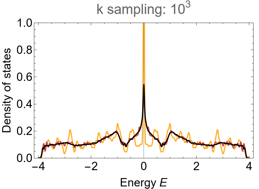
and the density of states can be computed by using the function ComputeEigenvalues, which can be found in the dropdown menu Needed function above.
(* Eigenvalues *)
evals = Association[# -> ComputeEigenvalues[Hclst[#], 10^3, 12, genusLst[#]] & /@ cells];

(* color maps *)
cLst = (ColorData["SunsetColors", "ColorFunction"] /@ (1 - Range[1, 3]/3.));

(* Visualize *)
SmoothHistogram[evals, 0.02, "PDF",
  Frame -> True, FrameLabel -> {"Energy E", "Density of states"} FrameStyle -> Black,
  ImageSize -> 500, ImagePadding -> {{Automatic, 10}, {Automatic, 10}}, LabelStyle -> 20,
  PlotLabel -> "k sampling: 10^2", PlotRange -> All, PlotStyle -> cLst]

\(\{6,4\}\)-BBH model#
The \(\{6,4\}\)-BBH model can be constructed by adjusting particular hopping amplitudes in the previously defined model. Our goal is to thread the lattice with magnetic \(\pi\)-fluxes through each cycle of orbitals as well as through each plaquette with alternating inter and intra-site hopping amplitudes.
We choose to adjust the intra-site coupling between orbital 1 and 4 by changing the sign of the hopping amplitude in the on-site terms. This introduces a \(\pi\)-flux through each cycle of orbitals:
onsiteInteractionMat = h0 {
    {  0,  1,  0, -1},
    {  1,  0,  1,  0},
    {  0,  1,  0,  1},
    { -1,  0,  1,  0}};

vertices = VertexList@pcmodel["Graph"];
onsitePC = AssociationThread[vertices ->
  ConstantArray[onsiteMassMat + onsiteInteractionMat, Length@vertices]];
where we have introduced a coupling constant h0 in order tune the intra-site coupling strength.
The above modification introduces \(\pi\)-fluxes through some plaquettes with alternating intra and inter-site hopping amplitudes in certain regions of the lattice. This implies that yet another modification is needed such that each plaquette is threaded by a \(\pi\)-flux. We can achieve this by adjusting the inter-site coupling between orbital 3 and 3 of another site by changing the sign of the inter-cell amplitudes in the hopping terms:
hopIntraCellMat = {
   {  0,  0,  0,  0},
   {  0,  0,  0,  1},
   {  0,  0, -1,  0},
   {  0,  0,  0,  0}};
We can assign the hopping amplitudes programmatically by iterating through the list of edge translations:
hoppingsVec = h1 If[# == "1", hopIntraCellMat, hopInterCellMat] & /@ pcmodel["EdgeTranslations"];
where we have introduced yet another a coupling constant h1 in order tune the inter-site coupling strength. Therefore:
edges = EdgeList@pcmodel["Graph"];
hoppingsPC = AssociationThread[edges -> hoppingsVec];
The Abelian Bloch Hamiltonians can be constructed as usual:
(* Hamiltonian for the primitive cell *)
Hpc = AbelianBlochHamiltonian[pcmodel, norbits &, onsitePC, hoppingsPC, CompileFunction -> True];

(* Hamiltonians for the supercells *)
Hsclst = Association[# ->
    AbelianBlochHamiltonian[scmodels[#], Norb &, onsitePC, hoppingsPC, PCModel -> pcmodel,
    CompileFunction -> True] &/@ cells[[2 ;;]]];

(* All *)
Hclst = Join[Association[cells[[1]] -> Hpc], Hsclst];
Three distinct phases can be identified by tuning the parameters:
phases = {"Topological phase", "Metallic phase", "Trivial phase"};
h0Lst = AssociationThread[phases, {0.5, 0.77, 1.5}];

evals = Association[
  Table[phase ->
    Association[# ->
      ComputeEigenvalues[Hclst[#] /. {h0 -> h0Lst[phase], h1 -> 1},  10^3, 8, genusLst[#]]
    &/@ cells],
  {phase, phases}]
];

Row[
 SmoothHistogram[evals[#], 0.02, "PDF",
    Frame -> True, FrameLabel -> {"Energy E", "Density of states"},
    FrameStyle -> Black,
    ImageSize -> 270,
    ImagePadding -> {{Automatic, 10}, {Automatic, 10}},
    LabelStyle -> 15,
    PlotLabel -> # <> "\nk sampling: 10^3, h0 = " <> ToString@h0Lst[[#]] <> "h1",,
    PlotRange -> {{-2, 2}, {-0.01, 1.01}}, PlotStyle -> cLst] & /@ phases,
 FrameMargins -> 0, ImageMargins -> 0]

Note that at the gap closing \(h_{0}=0.77 h_{1}\) the transition for small supercells appears semi-metallic with vanishing density of states at \(E=0\). However, the DOS converges to a finite value for larger supercells, which implies that this is a finite-size effect.
Finite flakes#
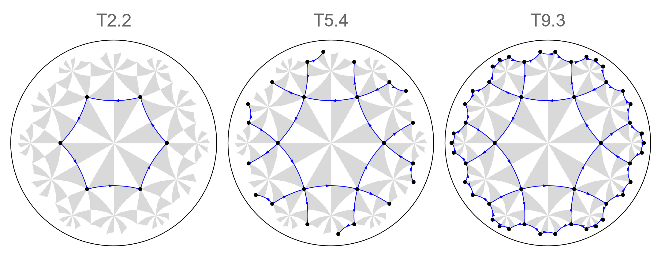
In order to demonstrate the bulk-boundary correspondence in the higher-order topological phase of the \(\{6,4\}\)-BBH model, we can repurpose the constructed sequence of supercell model graphs. Before we terminate the system to a finite size, let us visualize the flakes we want to consider. This can be achieved by turning off the display of inter-cell edges specified through the option ShowInterCellEdges within the option ShowCellGraphFlattened in the function VisualizeModelGraph[] by setting it to False:
Row[
  VisualizeModelGraph[cmodels[#],
    Elements -> <|
      ShowCellGraphFlattened -> {
        ShowVertexLabels -> False,
        ShowInterCellEdges -> False
        }
      |>,
    ImageSize -> 300,
    NumberOfGenerations -> 3,
    PlotLabel -> #, LabelStyle -> 20]
  & /@ cells]

The Abelian Bloch Hamiltonians of (supercell) model graphs depends on the chosen quasiparticle basis used by the HyperBloch package. The used convention is cell-dependent and thus hyperbolic momenta are introduced in inter-cell hopping terms. This enables us to construct the tight-binding Hamiltonians for finite flakes in real space efficiently by setting inter-cell terms to zero through the function TBHamiltonian:
HcFlakelst = Join[
  Association[
    cells[[1]] -> TBHamiltonian[cmodels[cells[[1]]], 4 &, onsitePC,
  hoppingsPC]],
  Association[
    # -> TBHamiltonian[cmodels[#], 4 &, onsitePC, hoppingsPC, PCModel -> cmodels[cells[[1]]]]
  & /@ cells[[2 ;;]]
]];
Next, let us calculate the spectra of the finite flakes by first computing the eigenvalues of the finite flakes:
evals = Association[# -> Eigenvalues[HcFlakelst[#] /. {h0 -> 0.1, h1 -> 1}] & /@ cells];
Then the spectra are given by:
Row[
 ListPlot[Sort[evals[#]],
    AxesOrigin -> {0, -2.5}, Frame -> True,
    FrameLabel -> {"n", "Energy E_n"}, FrameStyle -> Black,
    ImageSize -> 350, LabelStyle -> 20, PlotLabel -> #,
    PlotRange -> {Automatic, {-2.5, 2.5}}] & /@ cells
 ]

The gapped spectrum indicates emergent boundary modes in the topological phase.
Disclination defects#
The introduction of disclination defects enables us to demonstrate the existence of boundary modes and associated quantized fractional charges in higher-order topological insulators. The HyperBloch package provides a function for the construction of finite flakes with disclination defects. This is achieved through a cutting and glueing procedure known as the Volterra process.
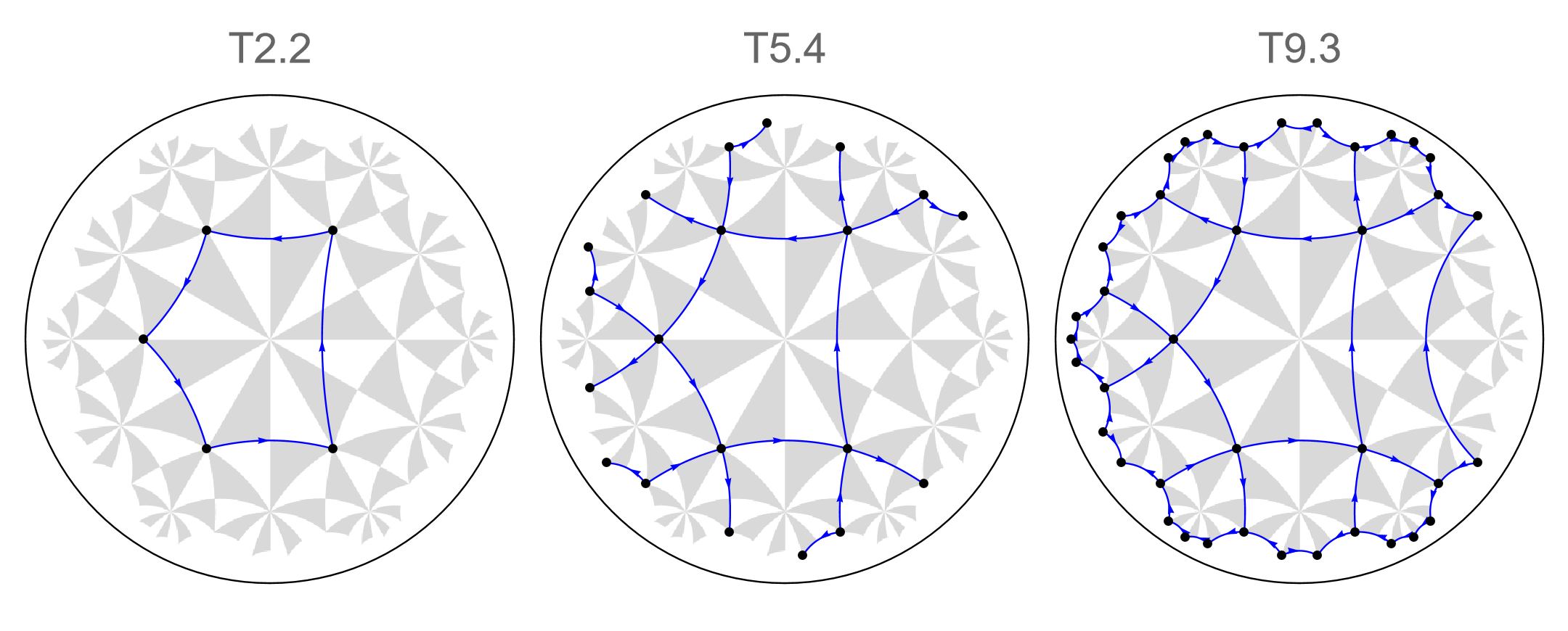
We choose to cut away a sector in the finite flake subtended by an angle \(\pi/3\), and glue the newly introduced borders together. The corresponding flakes can easily be constructed through the function IntroduceDisclination. To do so, we set the so-called Frank angle \(\alpha_{F}\) to \(-\pi/3\). This can be specified by passing a negative integer to the function, which we denote as the Frank angle increment \(\Delta\alpha_{F}\), taking values \(-1, -2, ... -(m-1)\), where \(m\) is given by the \(C_{m}\) rotation symmetry \(m \, \epsilon \, \{r, q, p\}\) specified by the chosen cell center. The actual Frank angle is then given by \(\alpha_{F} = \Delta\alpha_{F}\,2\pi/m\). In addition, a reference angle needs to be passed, which specifies the relative rotation angle in counter-clockwise direction of the normal vector to the reference vector \(\vec{v}=(1, 0)\) defining the disclination defect. Analogous to the Frank angle increments, the reference angle is specified by a positive integer, which we denote as the reference angle increment , taking values \(0, 1, 2, ... 2m-1\). A disclination defect can thus be introduced as follows:
cmodelsDisclination = Association[# -> IntroduceDisclination[cmodels[#], -1, 0] & /@ cells];
We can visualize the (supercell) model graphs with disclination defects using the function VisualizeModelGraph[]:
Row[
  VisualizeModelGraph[cmodelsDisclination[#],
    Elements -> <|
      ShowCellGraphFlattened -> {ShowVertexLabels -> False}
    |>,
    ImageSize -> 300,LabelStyle -> 20
    NumberOfGenerations -> 3, PlotLabel -> #]
  & /@ cells]

The newly introduced edges can be accessed through the key ”GluedEdges”. They inherit some of the labels originating from the (supercell) model graphs they are based on. Each glued edge carries an edge tag containing a list of the form { “g”, idx } where the string ”g” indicates that the edge is a glued edge and idx is a running index, indicating the position in the list of glued edges.
For example, for a model graph based on the T2.2 primitive cell the glued edges are given as:
cmodelsDisclination["T2.2"]["GluedEdges"]

and for model graph based on the T5.4 supercell the glued edges are given as:
cmodelsDisclination["T5.4"]["GluedEdges"]

Particular attention is required when assigning coupling constants for the construction of corresponding Hamiltonians. In general, every flake with a disclination defect should be considered individually due to the newly introduced GluedEdges.
First, let us consider the smallest flake associated with the T2.2 primitive cell. This is a rather trivial case, since all edges, including the GluedEdges, should be associated with intra-cell hopping amplitudes:
gluedEdges = cmodelsDisclination["T2.2"]["GluedEdges"];
hoppingsGlued = AssociationThread[gluedEdges -> {hopMat1}];
Every other coupling relation is inherited by the previously defined model on the primitive cell. The tight-binding Hamiltonian in real space can now be set up by specifying the model graph with a disclination defect, the model graph of the primitive cell without a disclination defect and the corresponding coupling constants specified above. These arguments are passed to the function TBHamiltonian as follows:
HPCDisclinationFlake = TBHamiltonian[
  cmodelsDisclination["T2.2"], cmodels["T2.2"], 4 &, onsitePC, hoppingsPC, hoppingsGlued
];
The workflow for the construction of tight-binding Hamiltonians of supercells with a disclination defect is unchanged:
hoppingsGlued = AssociationThread[
  cmodelsDisclination["T5.4"]["GluedEdges"] -> {hopMat1}
];

HSC1DisclinationFlake = TBHamiltonian[
  cmodelsDisclination["T5.4"], cmodels["T2.2"], 4 &, onsitePC, hoppingsPC, hoppingsGlued
];
We can repeat this procedure for every consecutive supercell:
hoppingsGlued = AssociationThread[
  cmodelsDisclination["T9.3"]["GluedEdges"] -> {hopMat1, hopMat2}
];

HSC2DisclinationFlake = TBHamiltonian[
  cmodelsDisclination["T9.3"], cmodels["T2.2"], 4 &, onsitePC, hoppingsPC, hoppingsGlued
];
It is convenient to collect everything:
HcDisclinationFlakelst = AssociationThread[cells,
  {HPCDisclinationFlake, HSC1DisclinationFlake, HSC2DisclinationFlake}];
The spectra are given by:
evals = Association[# -> Eigenvalues[HcDisclinationFlakelst[#] /. {h0 -> 0.1, h1 -> 1}] & /@ cells];

Row[
 ListPlot[Sort[evals[#]],
    AxesOrigin -> {0, -2.5}, Frame -> True,
    FrameLabel -> {"n", "Energy E_n"}, FrameStyle -> Black,
    ImageSize -> 350, LabelStyle -> 20, PlotLabel -> #,
    PlotRange -> {Automatic, {-2.5, 2.5}}] & /@ cells
 ]

We can compare the visualized spectra with the previous ones for the flakes without disclination defects. The emergence of the new in-gap states implies a filling anomaly and indicates quantized fractional charges. Let us explicitly emphasize some of these in-gap states:
inGapStates = AssociationThread[cells,
  {{{12.5, 14.5}, {0.59, 0.63}}, {{57.5, 59.5}, {0.59, 0.63}}, {{92.5, 94.5}, {0.59, 0.63}}}];
subPlotPosX = AssociationThread[cells, {{5, 1.25}, {20, 1.25}, {38, 1.25}}];

Row[
 ListPlot[Sort[evals[#]],
    AxesOrigin -> {0, -2.5}, Frame -> True,
    FrameLabel -> {"n", "Energy E_n"}, FrameStyle -> Black,
    ImageSize -> 350, LabelStyle -> 20, PlotLabel -> #,
    PlotRange -> {Automatic, {-2.5, 2.5}},

    Epilog -> Inset[
      ListPlot[Sort[evals[#]],
       Frame -> True, ImageSize -> Scaled[130],
       PlotRange -> inGapStates[#],
       PlotStyle -> Directive[Red, PointSize[Medium]]
       ], subPlotPosX[#]]
    ] & /@ cells
 ]

Visualizing the Volterra process (bonus)#
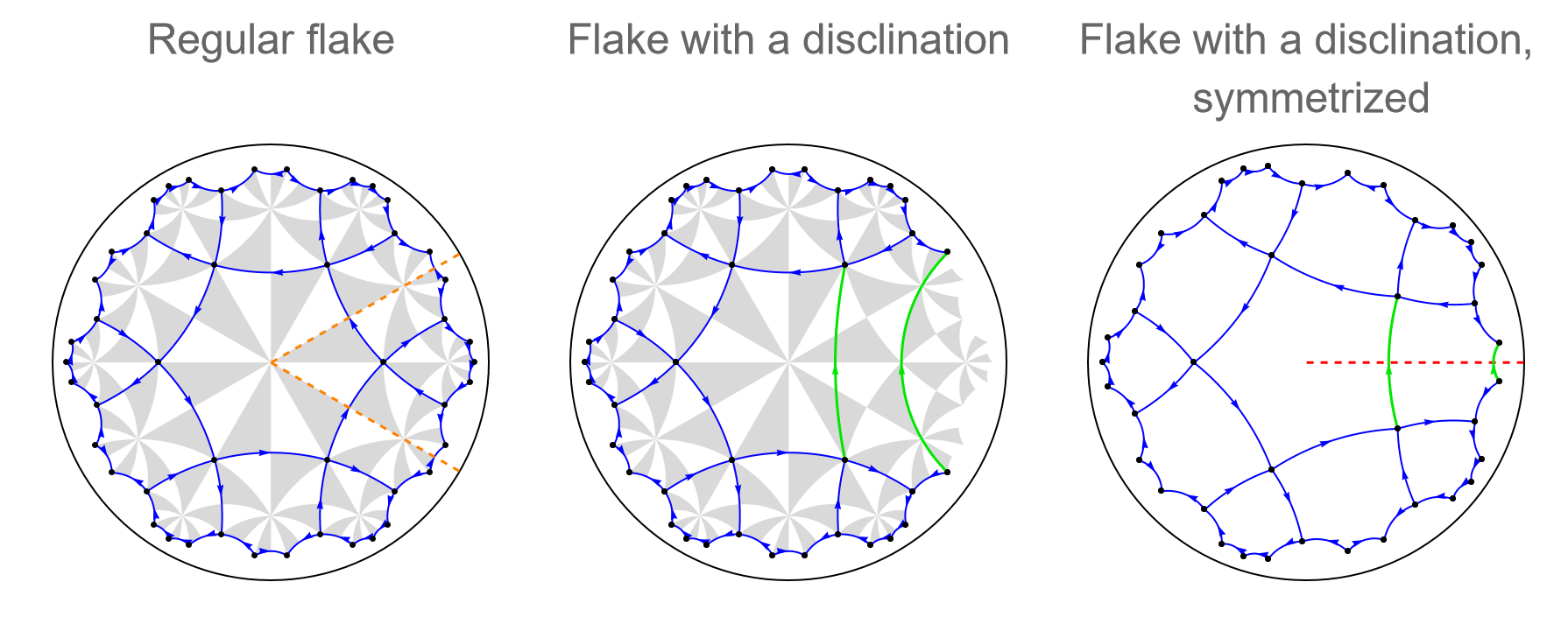
We can visualize the Volterra process step by step.
For example, let us consider the T9.3 supercell. A sector subtended by an angle \(\pi/3\) is cut out of the T9.3 supercell. The cut out wedge lies within the region specified by the following two lines:
FrankAngle = cmodelsDisclination["T9.3"]["FrankAngle"];
referenceAngle = cmodelsDisclination["T9.3"]["ReferenceAngle"];

upperCut = Line[{{0, 0}, Dot[RotationMatrix[referenceAngle], RotationMatrix[Abs[FrankAngle/2]], {1, 0}]}];
bottomCut = Line[{{0, 0}, Dot[RotationMatrix[referenceAngle], RotationMatrix[FrankAngle/2], {1, 0}]}];
The regular flake together with the two cuts can be visualized as follows :
regularFlake = Show[
   VisualizeModelGraph[cmodels["T9.3"],
    NumberOfGenerations -> 3,
    Elements -> <|
      ShowCellGraphFlattened -> {
        ShowVertexLabels -> False, ShowInterCellEdges -> False,
        CellVertexStyle -> Directive[Black, AbsolutePointSize[3]]
        }
      |>
    ],
   Graphics[{Orange, Dashed, AbsoluteThickness[1.5], upperCut}],
   Graphics[{Orange, Dashed, AbsoluteThickness[1.5], bottomCut}],
   ImageSize -> 300, LabelStyle -> 20,
   PlotLabel -> "Regular flake\n"];
The disclination and the glued edges can be visualized using the high-level visualization function VisualizeModelGraph:
disclinationFlake = Show[
   VisualizeModelGraph[cmodelsDisclination["T9.3"],
    NumberOfGenerations -> 3,
    Elements -> <|
      ShowCellGraphFlattened -> {
        ShowVertexLabels -> False,
        CellVertexStyle -> Directive[Black, AbsolutePointSize[3]],
        EdgeFilter -> (#[[3, 3, 2, 1, 1 ]] != "g" &)}
      |>
    ],
   ShowCellGraphFlattened[cmodelsDisclination["T9.3"],
    ShowVertexLabels -> False,
    IntraCellEdgeStyle ->
     Directive[Darker[Green, 0.1], AbsoluteThickness[1.5]],
    CellVertexStyle -> Directive[Black, AbsolutePointSize[3]],
    EdgeFilter -> (#[[3, 3, 2, 1, 1 ]] == "g" &)
    ],
   ImageSize -> 300, LabelStyle -> 20,
   PlotLabel -> "Flake with a disclination\n"];
It is possible to symmetrize the resulting flake using the option SymmetrizeFlake of IntroduceDisclination:
cmodelsDisclinationSymmetric =
  Association[# ->
      IntroduceDisclination[cmodels[#], -1, 0,
       SymmetrizeFlake -> True] & /@ cells];
The disclination defect can explicitly be indicated using the options IndicateDisclination and DisclinationLineStyle of VisualizeModelGraph:
disclinationFlakeSymmetrized = Show[
   VisualizeModelGraph[cmodelsDisclinationSymmetric["T9.3"],
    NumberOfGenerations -> 3,
    IndicateDisclination -> True,
    DisclinationLineStyle -> Directive[Red, Dashed, AbsoluteThickness[1.5]],
    Elements -> <|
      ShowCellGraphFlattened -> {
        ShowVertexLabels -> False,
        CellVertexStyle -> Directive[Black, AbsolutePointSize[3]],
        EdgeFilter -> (#[[3, 3, 2, 1, 1 ]] != "g" &)}
      |>
    ],
   ShowCellGraphFlattened[cmodelsDisclinationSymmetric["T9.3"],
    ShowVertexLabels -> False,
    IntraCellEdgeStyle ->
     Directive[Darker[Green, 0.1], AbsoluteThickness[1.5]],
    CellVertexStyle -> Directive[Black, AbsolutePointSize[3]],
    EdgeFilter -> (#[[3, 3, 2, 1, 1 ]] == "g" &)
    ],
   ImageSize -> 300, LabelStyle -> 20,
   PlotLabel -> "Flake with a disclination,\n symmetrized"];
Finally, let us put everything together:
Row[{regularFlake, disclinationFlake, disclinationFlakeSymmetrized}]


