Flat-bands#

The HyperCells package contains built-in functions for several tight-binding models such as:

TessellationModelGraph which constructs a tessellation graph from a cell graph of a triangle group, i.e. the nearest-neighbor graphs of the \(\{p,q\}\)-tesselation of the hyperbolic plane.
LiebModelGraph which constructs a Lieb graph from a cell graph of a triangle group.
KagomeModelGraph which constructs a kagome graph from a cell graph of a triangle group.
TGCellModelGraph which constructs a model graph from a cell graph and a specification of which cell-graph vertices are to be used as vertices of the model graph, which define edges, and which define faces of the model graph.

as well as :

AddOrientedNNNEdgesToTessellationModelGraph which modifies the \(\{p,q\}\)-tesselation model graph model by adding oriented next-nearest neighbor edges to all faces with at least five edges.

Previously, in the tutorials Getting started with the HyperBloch and Supercells, we have constructed tessellation graphs. In this tutorial we will construct hyperbolic Lieb lattices and hyperbolic kagome lattices on primitive cells and supercells. Both constructions rely on the TGCellModelGraph function which we will discuss afterwards.

Skip to page Haldane model

The construction of next-nearest-neighbor model graphs through the function AddOrientedNNNEdgesToTessellationModelGraph will be discussed in the next tutorial on hyperbolic Haldane models.

\(\{6,4\}\)-Lieb lattice#

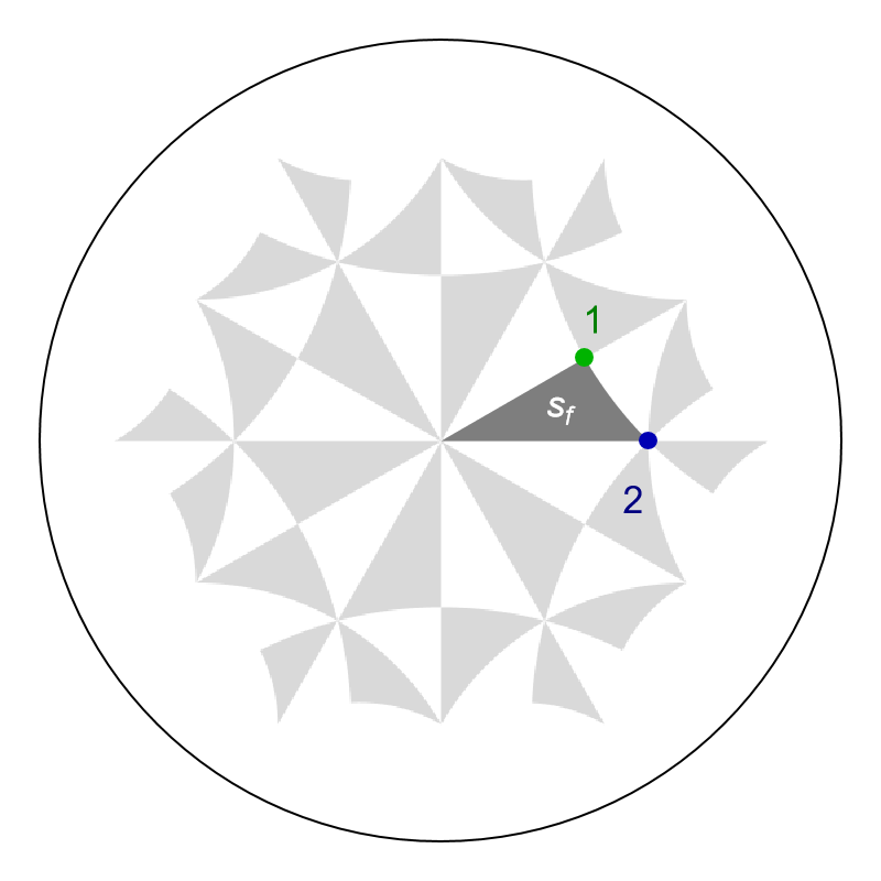
Hyperbolic Lieb lattices are specified by placing vertices at Wyckoff positions 1 and 2 for \(\{p,q\}\)-tesselations of the hyperbolic plane (here we choose 1 and 2 corresponding to the x and y vertices of the fundamental Schwarz triangle). It is instructive to jump a bit ahead to look at the two Wyckoff positions and the fundamental Schwarz in the Poincaré disk, which we will properly discuss shortly after:

Next, let us start by constructing a cell graph on the primitive cell for the \(\{6,4\}\)-lattice in GAP:

# Primitive cell:
# ---------------
tg := ProperTriangleGroup( [ 2, 4, 6 ] );
qpc := TGQuotient( 1, [ 2, 4, 6 ] );
cgpc := TGCellGraph( tg, qpc, 3 : simplify := 5 );
Export( cgpc, "(2,4,6)_T2.2_3.hcc" ); # export

Analogous to the TessellationModelGraph function, all built-in model graph functions only need to be specified on the primitive cell. The model specifications are inherited by subsequent supercell model graphs. The Lieb lattice can be constructed as follows:

# Lieb lattice:
# -------------
# elementary nearest-neighbor model
model_Lieb := LiebModelGraph( cgpc );
Export( model_Lieb, "{6,4}-Lieb_T2.2_3.hcm" ); # export

We choose a supercell sequence by following the central concepts discussed in the tutorial Supercells and Coherent sequences:

# Supercells:
# -----------
tgQS := TGQuotientSequencesStructure(tg : boundByGenus := 10);;
sequence := LongestSequence(tgQS : quotient := 1);
sc_lst := sequence{[2..Length(sequence)]};

for sc_i_index in sc_lst do

  qsc_i := TGQuotient( sc_i_index );
  sc_i := TGCellSymmetric(tg, qsc_i, 3);
  scmodel_i := TGSuperCellModelGraph(model_Lieb, sc_i);
  
  sc_i_label := StringFormatted("_T2.2_3_sc-T{}.{}.hcs", sc_i_index[1], sc_i_index[2]);
  scmodel_i_name := JoinStringsWithSeparator(["{6,4}-Lieb", sc_i_label], "");
  Export(scmodel_i,  scmodel_i_name); # export
od;

Download generated files Download GAP Code

Next, in Mathematica we load the HyperBloch package, set the working directory of the files we have created through the HyperCells package and in addition define a list of available unit cells together with the corresponding genera of the compactified unit cells:

(* Preliminaries *)
<< PatrickMLenggenhager`HyperBloch`
SetDirectory[NotebookDirectory[]];

cellsLieb = {"T2.2", "T5.4", "T9.3"}; 
genusLstLieb = {2, 5, 9};

The cell, model and supercell model graph can now be imported by parsing the imported strings with the functions ImportCellGraphString, ImportModelGraphString and ImportSupercellModelGraphString, respectively:

(* Primitive cell *)
pcellLieb = ImportCellGraphString[Import["(2,4,6)_T2.2_3.hcc"]];
pcmodelLieb = ImportModelGraphString[Import["{6,4}-Lieb_T2.2_3.hcm"]];

(* Import supercells *)
scmodelsLieb = Association[# -> 
  ImportSupercellModelGraphString[ 
    Import["{6,4}-Lieb_T2.2_3_sc-" <> # <> ".hcs"]] 
  &/@ cellsLieb[[2 ;;]]];

It is instructive to visualize the graph representation of the model in the primitive cell after the model graph has been imported. Moreover, we choose to highlight the two Wyckoff positions and the fundamental Schwarz in the Poincaré disk.

We can visualize Wyckoff positions of the fundamental Schwarz triangle through the function GetWyckoffPosition, which enables us to extract the corresponding coordinates in the Poincaré disk, where we will use the label ”1” that identifies the symmetry operation relating the vertices of the fundamental Schwarz triangle to the Wyckoff positions:

x = GetWyckoffPosition[{2, 4, 6}, {1, "1"}];
y = GetWyckoffPosition[{2, 4, 6}, {2, "1"}];

We can highlighted individual Schwarz triangles in the Poincaré disk through the function GetSchwarzTriangle. Let us extract the Polygon representing the fundamental Schwarz triangle associated with the identity element in the proper triangle group \(\Delta^{+}(2,4,6)\):

sf = GetSchwarzTriangle[{2, 4, 6}, "1"];

We can highlight the two Wyckoff positions and the fundamental Schwarz triangle in the graph representation of the nearest-neighbor tight-binding model model as follows:

Show[
 VisualizeModelGraph[pcmodelLieb,
  CellGraph -> pcellLieb,
  NumberOfGenerations -> 3,
  Elements -> <|
    	ShowCellGraphFlattened -> {},
    	ShowCellBoundary -> {ShowEdgeIdentification -> True}
    |>],
 
 Graphics[{Darker[Gray, 0.01], Opacity[0.4], sf}],
 Graphics[{Text[Style["s_f", 17, Thick, White], {0.3, 0.09}]}],
 
 Graphics[{Darker[Green, 0.3], PointSize[0.03], Point@x}],
 Graphics[{Darker[Blue, 0.3], PointSize[0.03], Point@y}],
 
 Graphics[{Darker[Green, 0.5], Text[Style["1", 17, Thick], {0.30, 0.17}]}],
 Graphics[{Darker[Blue, 0.5], Text[Style["2", 17, Thick], {0.43, 0.00}]}],
 
 ImageSize -> 400
 ]

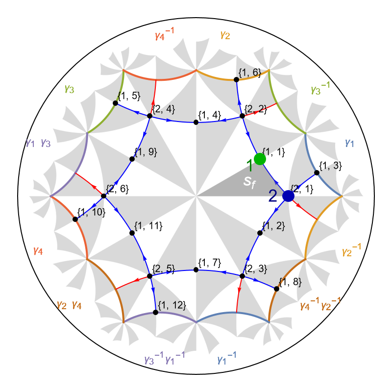
Unlike the edge tags of tesselation and kagome model graphs, see Getting started with the HyperBloch package, the edge tags of Lieb models graphs are of a reduced form. Let us take a look at the edges in the model graph:

EdgeList@pcmodelLieb["Graph"]

Each element in the list is a DirectedEdge, connecting a pair of vertices. The EdgeTags (the list above the arrows) for the nearest-neighbour edges take the form {1, s}, where the first entry, 1, indicates a nearest-neighbor edge, and s is the position of the Schwarz triangle associated with the cell-graph edges in \(T_{\Delta^{+}}(\Gamma)\).

Once the (supercell) model graphs are imported the corresponding Abelian Bloch Hamiltonians for the elementary nearest-neighbor hopping model can be constructed. We set the number of orbital per site to one, the on-site terms \(0\) and the nearest-neighbor hopping amplitudes to \(-1\):

(* primitive cell *)
HpcLieb = AbelianBlochHamiltonian[pcmodelLieb, 1, 0 &, -1 &, CompileFunction -> True];

(* supercells *)
HscLieblst = Association[# -> 
  AbelianBlochHamiltonian[scmodelsLieb[#], 1, 0 &, -1 &, PCModel -> pcmodelLieb, CompileFunction -> True] 
  &/@ cellsLieb[[2 ;;]] ];

(* all *)
HcLieblst = Join[Association[cellsLieb[[1]] -> HpcLieb], HscLieblst];

The supercell method can be applied as usual, where we use the function ComputeEigenvalues, which can be found in the dropdown menu Needed function above:

(* color maps *)
cLst = (ColorData["SunsetColors", "ColorFunction"] /@ (1 - Range[1, 3]/3.));

(* Compute the Eigenvalues *)
evalsLieb = Association[# ->  ComputeEigenvalues[HcLieblst[#], 10^4, 32, genusLstLieb[#]]&/@cellsLieb];

(* Visualize *)
SmoothHistogram[evalsLieb, 0.01, "PDF",
  Frame -> True, FrameLabel -> {"Energy E", "Density of states"} FrameStyle -> Black, 
  ImageSize -> 500, ImagePadding -> {{Automatic, 10}, {Automatic, 10}}, LabelStyle -> 20,
  PlotLabel -> "k sampling: 10^4", PlotRange -> All, PlotStyle -> cLst]

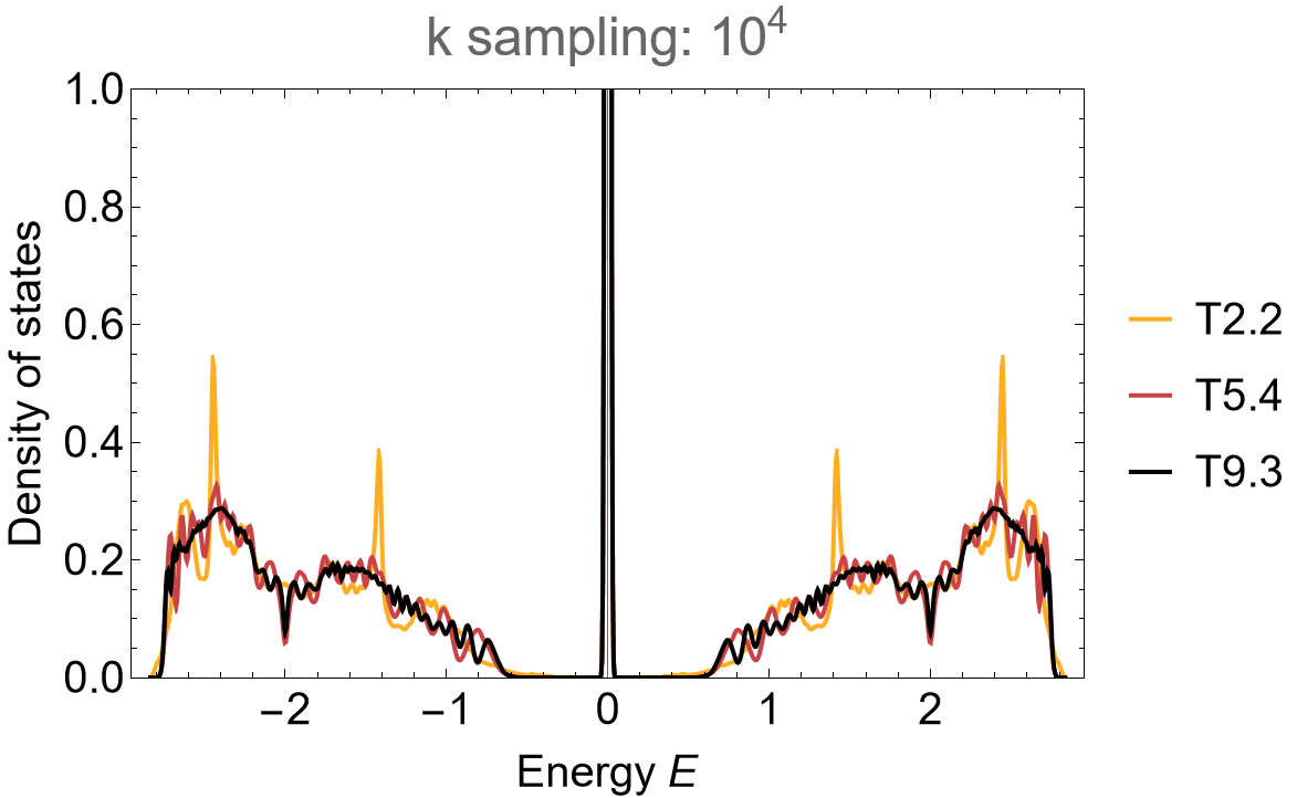
Pronounced flat-bands emerge in density of states, centered around zero energy with gaps developing between the flat-band and the dispersive part of the spectrum.

Download Mathematica Notebook

\(\{8,3\}\)-kagome lattice#

Hyperbolic kagome lattices can be constructed just as easily as hyperbolic Lieb lattices. These lattices are specified by placing vertices at Wyckoff positions 1. These lattices are restricted to \(\{p,3\}\)-tesselation of the hyperbolic plane. Once again, we start by constructing the cell graph and model graph for the primitive cell in GAP:

# Primitive cell:
# ---------------
tg := ProperTriangleGroup( [ 2, 3, 8 ] );
qpc := TGQuotient( 1, [ 2, 3, 8 ] );
cgpc := TGCellGraph( tg, qpc, 3 : simplify := 5 );
Export( cgpc, "(2,3,8)_T2.1_3.hcc" ); # export

The kagome lattice can be constructed as follows:

# Kagome lattice:
# ---------------
model_kagome := KagomeModelGraph( cgpc );
Export( model_kagome, "{8,3}-kagome_T2.1_3.hcm" ); # export

with supercells:

# Supercells:
# -----------
tgQS := TGQuotientSequencesStructure(tg : boundByGenus := 20);;
sequence := LongestSequence(tgQS : quotient := 1);
sc_lst := sequence{[2..Length(sequence)]};

for sc_i_index in sc_lst do

  qsc_i := TGQuotient( sc_i_index );
  sc_i := TGCellSymmetric(tg, qsc_i, 3);
  scmodel_i := TGSuperCellModelGraph(model_kagome, sc_i);

  sc_i_label := StringFormatted("_T2.1_3_sc-T{}.{}.hcs", sc_i_index[1], sc_i_index[2]);
  scmodel_i_name := JoinStringsWithSeparator(["{8,3}-kagome", sc_i_label], "");
  Export(scmodel_i,  scmodel_i_name); # export
od;

Download generated files Download GAP Code

We can proceed anologously to the hyperbolic Lieb lattice in Mathematica, we omitt the detailed specificities which can be found in the downloadable files. As such, let us visualize the \(\{8,3\}\)-kagome lattice:

VisualizeModelGraph[pcmodelKagome,
  CellGraph -> pcellKagome,
  Elements -> <|
        ShowCellGraphFlattened -> {},
   	ShowCellBoundary -> {ShowEdgeIdentification -> True}
  |>,
  ImageSize -> 400,
  NumberOfGenerations -> 3]

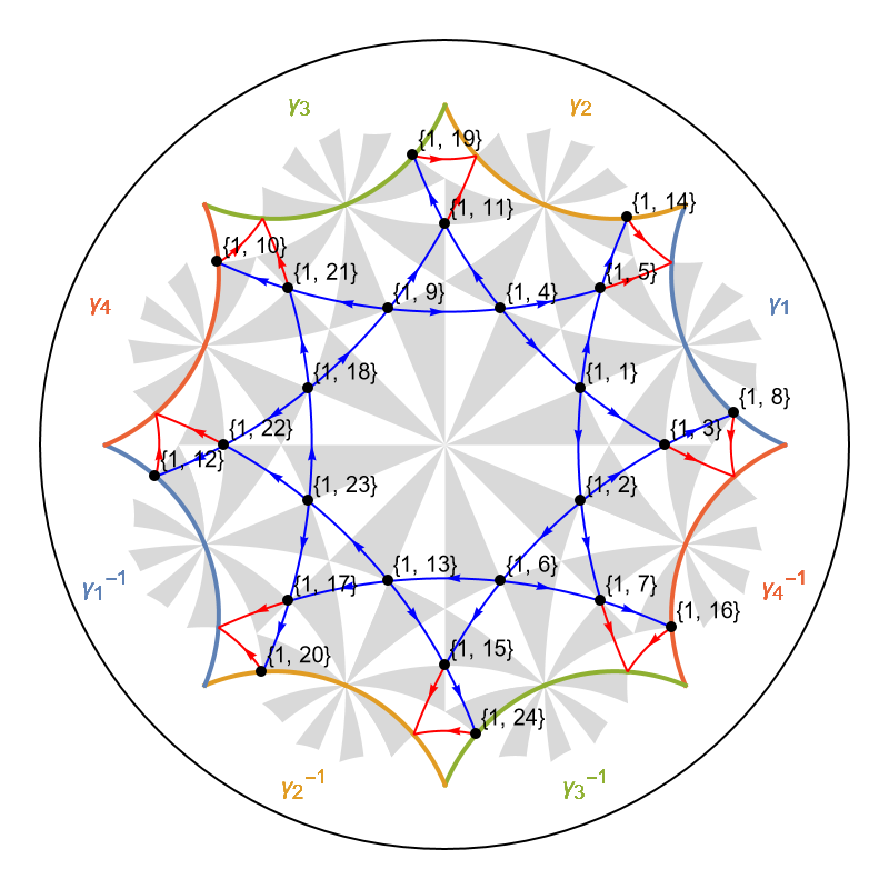
The application of the supercell method shows a fast convergence to the thermodynamic limit in the density of states:

dos = SmoothHistogram[evalsKagome, 0.01, "PDF",
  Frame -> True, FrameLabel -> {"Energy E", "Density of states"} FrameStyle -> Black, 
  ImageSize -> 500, ImagePadding -> {{Automatic, 10}, {Automatic, 10}}, LabelStyle -> 20,
  PlotLabel -> "k sampling: 2*10^4", PlotRange -> All, PlotStyle -> cLst]

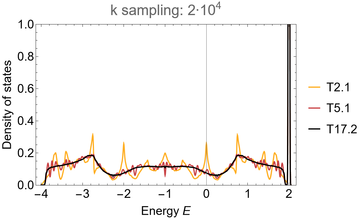
The density of states for the \(\{8,3\}\)-lattice exhibits pronounced flat-band centered at \(E=2\) with gaps developing between the flat-band and the dispersive part of the spectrum. The accumulation of higher-dimensional irreducible representations on the primitive cell through the supercell method comes with a characteristic density of states suppression near the edges. As such, let us take a closer look at the band edge in the vicinity of the flat-band:

Show[dos,
 Epilog -> {
   Inset[Show[First@dos,
     FrameLabel -> None, Frame -> True, ImageSize -> 200,
     LabelStyle -> 15, PlotRange -> {{1.85, 2.05}, {0, 0.4}},
     PlotLabel -> None], {-2, 0.65}]
   }]

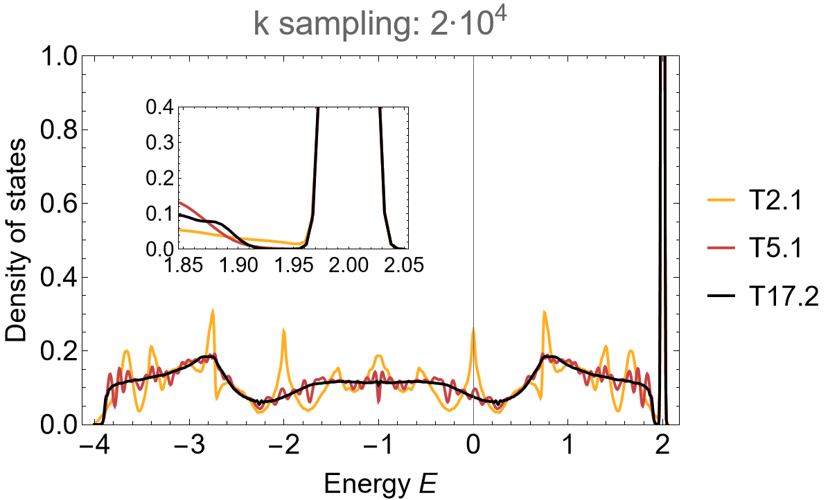
The density of states between the flat-band and the dispersive bands is suppressed with increasing supercell size, such that in the thermodynamic limit the flat-band is detached. This suggests that the gaplessness for the primitive cell is a finite-size effect.

Download Mathematica Notebook