Hatano-Nelson model#
Learning goals
Construction of non-Hermitian Abelian Bloch Hamiltonians of:
a tight-binding model with Hermiticity-breaking gains and losses
and a variant of the Hatano-Nelson model for the \(\{6,4\}\)-lattice.
Featured functions
HyperCells:
Export, LongestSequence, ProperTriangleGroup, TGCellSymmetric, TessellationModelGraph, TGQuotient, TGQuotientSequencesStructure, TGSuperCellModelGraph
HyperBloch:
AbelianBlochHamiltonian, GetCellGraphEdge, ImportCellGraphString, ImportModelGraphString, ImportSupercellModelGraphString, NonReciprocalAbelianBlochHamiltonian, ShowCellBoundary, ShowCellGraphFlattened, VisualizeModelGraph
Needed functions
Mathematica:
In previous tutorials, such as Getting started with the HyperBloch package and HyperBloch Supercells tutorial etc., we have calculated the density of states of various nearest-neighbor tight-binding models via exact diagonalization and random samples. We predefine a function in order to calculate the eigenvalues for the (non-reciprocal) Abelian Bloch Hamiltonians that we will construct. We take advantage of the independence of different momentum sectors and parallelize the computation, where we partition the set of Npts into Nruns subsets:
ComputeEigenvalues[cfH_, Npts_, Nruns_, genus_] :=
 Flatten@ParallelTable[
   Flatten@Table[
     Eigenvalues[cfH @@ RandomReal[{-Pi, Pi}, 2 genus]],
    {i, 1, Round[Npts/Nruns]}], {j, 1, Nruns},
  Method -> "FinestGrained"]
The HyperBloch package provides a framework for the construction of Abelian Bloch Hamiltonians of Hermitian as well as non-Hermitian systems. In principle, the workflow for the construction of non-Hermitian compared to Hermitian models is unchanged. However, particular attention is required when assigning coupling constants. In this tutorial we will see how non-Hermitian hyperbolic lattice models can be set up through the construction of nearest-neighbor tight-binding models on the \(\{6,4\}\)-lattice. Specifically, we will consider Hermiticity-breaking terms, such as gains and losses, and a variant of the Hatano-Nelson model.
Prerequisits#
In order to construct the Abelian Bloch Hamiltonian for the two non-Hermitian models, we need to create the necessary files using the HyperCells package in GAP:
# load the HyperCells package
LoadPackage( "HyperCells" );
tg := ProperTriangleGroup( [ 2, 4, 6 ] );

# Primitive cell:
# ---------------
qpc := TGQuotient( 1, [ 2, 4, 6 ] );
cgpc := TGCellGraph( tg, qpc, 3 : simplify := 5 );
Export( cgpc, "(2,4,6)_T2.2_3.hcc" ); # export

# specify underlying model graph
model := TessellationModelGraph(cgpc);
Export(model, "{6,4}-tess-NN_T2.2_3.hcm");
We choose a supercell sequence by following the central concepts discussed in the tutorial Supercells and Coherent sequences. The model specifications are inherited by subsequent supercell model graphs:
# Supercells:
# -----------
tgQS := TGQuotientSequencesStructure(tg : boundByGenus := 10);;
sequence := LongestSequence(tgQS : quotient := 1);
sc_lst := sequence{[2..Length(sequence)]};

for sc_i_index in sc_lst do
    qsc_i := TGQuotient( sc_i_index );

    sc_i := TGCellSymmetric(tg, qsc_i, 3);
    scmodel_i := TGSuperCellModelGraph(model, sc_i);

    sc_i_label := StringFormatted("_T2.2_3_sc-T{}.{}.hcs", sc_i_index[1], sc_i_index[2]);
    scmodel_i_name := JoinStringsWithSeparator(["{6,4}-tess-NN", sc_i_label], "");
    Export(scmodel_i,  scmodel_i_name); # export file
od;
As usual, we load the HyperBloch package, set the working directory of the files we have created through the HyperCells package, define a list of available unit cells together with the corresponding genera of the compactified unit cells and import the cell, model and supercell model graph:
(* Preliminaries *)
<< PatrickMLenggenhager`HyperBloch`
SetDirectory[NotebookDirectory[]];

(* Labels and genera *)
cells = {"T2.2", "T5.4", "T9.3"};
genusLst = {2, 5, 9};

(* Import cell and model graph of the primitive cell *)
pcell = ImportCellGraphString[Import["(2,4,6)_T2.2_3.hcc"]];
pcmodel = ImportModelGraphString[Import["{6,4}-tess-NN_T2.2_3.hcm"]];

(* Import supercell model graph *)
scmodels = Association[# ->
    ImportSupercellModelGraphString[Import["{6,4}-tess-NN_T2.2_3_sc-" <> # <> ".hcs"]]
  &/@cells[[2 ;;]]];
It is instructive to visualize the \(\{6,4\}\)-tesselation model graph in order to properly assign the coupling constants:
VisualizeModelGraph[pcmodel,
	CellGraph -> pcell,
	Elements -> <|
		ShowCellGraphFlattened -> {},
		ShowCellBoundary -> {ShowEdgeIdentification -> True}
	|>,
  ImageSize -> 300,
  NumberOfGenerations -> 3]

Non-Hermitian on-site terms#
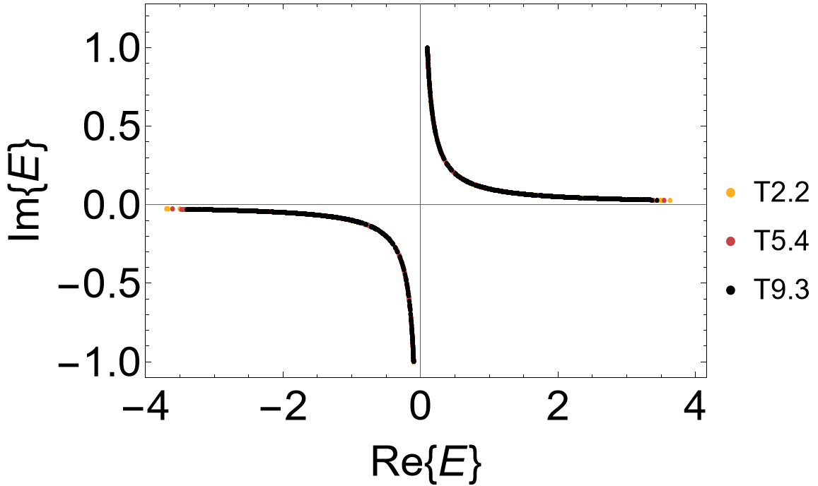
We choose to endow the \(\{6,4\}\)-lattice with gains and losses by introducing a staggered complex on-site potential. Since the hyperbolic hexagons have an even number of sides the lattice can be considered as bipartite such that a sublattice mass can be realized with \(\pm (M + i \eta)\). It is instructive to take a look at the list of vertices in the model graph in order to identify the sub-lattices:
VertexList@pcmodel["Graph"]

Comparing the list of vertices with the model representation we have previously visualized, we can assign the staggered on-site potential as follows:
mVec = (M + I eta) {1, -1, -1, 1, 1, -1};
onsitePC = AssociationThread[VertexList@pcmodel["Graph"] -> mVec];
The non-Hermitian Abelian Bloch Hamiltonians with complex staggered on-site potentials can be constructed through the AbelianBlochHamiltonian function, where we set the nearest-neighbor hopping amplitudes to -1:
Hpc = AbelianBlochHamiltonian[pcmodel, 1, onsitePC, -1 &, CompileFunction -> True];
and correspondingly for the supercells:
Hsclst = Association[# ->
    AbelianBlochHamiltonian[scmodels[#], 1, onsitePC, -1 &, PCModel -> pcmodel, CompileFunction -> True]
  &/@cells[[2 ;;]]];
For convenience, let us collect the constructed Hamiltonians in one Association:
Hclst = Join[Association[cells[[1]] -> Hpc], Hsclst];
The supercell method can be applied as usual, where we use the function ComputeEigenvalues, which can be found in the dropdown menu Needed function above:
evals = Association[# ->
    ComputeEigenvalues[Hclst[#] /. {M -> 0.1, eta -> 1}, 10^4, 32, genusLst[#]]
  &/@cells];
The complex spectrum can be visualized by using the built-in function ComplexListPlot of Mathematica. However, this might take a few minutes to be displayed. As such let us thin down our data sets by taking smaller subsets through random samples:
ComplexRandomThinning[evs_, Npts_] := Module[{keys},
  keys = Keys[evs];
  Association[
   Table[key -> RandomSample[Flatten[evs[key]], Npts],
    {key, keys}]]]
The complex spectrum exhibits a line gap:
(* color maps *)
cLst = (ColorData["SunsetColors", "ColorFunction"] /@ (1 - Range[1, 3]/3.));

ComplexListPlot[ComplexRandomThinning[evals, 1000],
 AspectRatio -> 1/1.5, Frame -> True, FrameLabel -> {"Re{E}", "Im{E}"},
 FrameStyle -> Directive[Black, 30], ImageSize -> 500, LabelStyle -> 20,
 PlotMarkers -> {"\[FilledCircle]", Scaled[0.015]},
 PlotRange -> {{-4, 4}, {-1.1, 1.1}}, PlotStyle -> cLst]

\(\{6,4\}\)-Hatano-Nelson model#
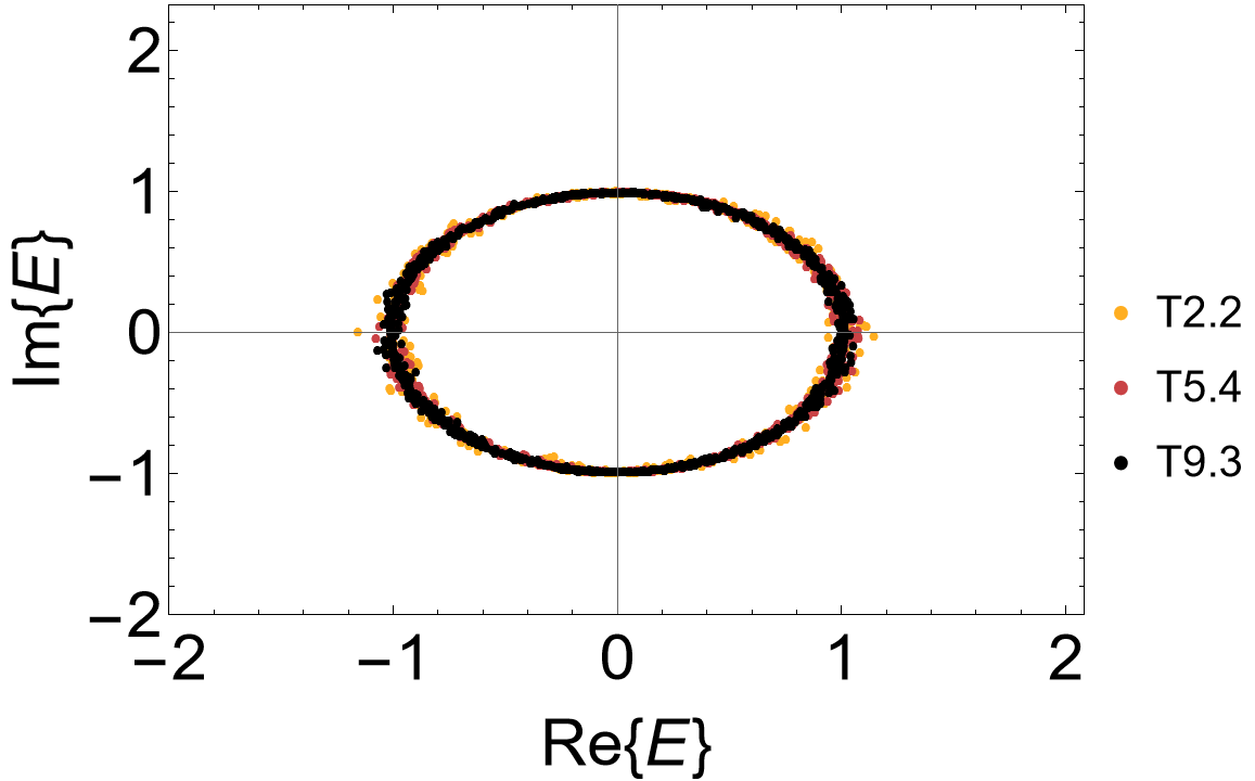
Other Hermiticity-breaking terms, aside from gains and losses, are for example non-reciprocal hopping amplitudes, most prominently used in the Hatano-Nelson model for a Euclidean one dimensional system with asymmetric hopping terms. A possible variant of the Hatano-Nelson model for the \(\{6,4\}\)-lattice consists of (weakly) coupled 1 dimensional chains with asymmetric hopping amplitudes and zero on-site potential. Each chain follows a hyperbolic geodesic and consists of a particular pair of vertices connected through directed edges in the model graph. Let us take a look at the list of edges in order to construct it:
EdgeList@pcmodel["Graph"]

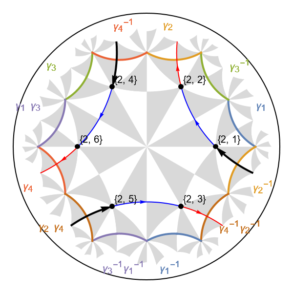
We choose to asymmetrically couple the vertices {{2,1},{2,2}}, {{2,3},{2,5}} and {{2,4},{2,6}}. It is helpful to visualize the corresponding directed edges in the model graph by first defining the list:
edgesInChains = {
    DirectedEdge[{2,1}, {2,2}], DirectedEdge[{2,2}, {2,1}],
    DirectedEdge[{2,3}, {2,5}], DirectedEdge[{2,5}, {2,3}],
    DirectedEdge[{2,4}, {2,6}], DirectedEdge[{2,6}, {2,4}]}
We can make use of the option EdgeFilter within the option ShowCellGraphFlattened in the function VisualizeModelGraph in order to visualize the corresponding one dimensional chains. Therefore, the graph representation of the Hatano-Nelson with decoupled one dimensional chains on the primitive cell looks as follows:
HNgraph = VisualizeModelGraph[pcmodel,
 CellGraph -> pcell,
 Elements -> <|
   ShowCellGraphFlattened -> {EdgeFilter -> (MemberQ[edgesInChains, #[[{1, 2}]]] &)},
   ShowCellBoundary -> {ShowEdgeIdentification -> True}
   |>,
  ImageSize -> 300,
  NumberOfGenerations -> 3]

It is instructive to also visualize the equivalent (translated) inter-cell edges starting outside the cell and ending inside. First, let us extract the inter-cell edges. Each inter-cell edge is associated with a non-trivial translation:
pcmodel["EdgeTranslations"]

In addition, we restrict the list to the edges present in the Hatano-Nelson chains specified in our previously defined list:
intercedges = Select[
    Transpose[{EdgeList@pcmodel["Graph"], pcmodel["EdgeTranslations"]}],
    MemberQ[edgesInChains, #[[1, {1, 2}]]] && #[[2]] != "1" &][[;;, 1]
  ];
We can use the function GetCellGraphEdge and its option ShowEquivalentEdge in order visualize specific edges and equivalent (translated) inter-cell edges in the Poincaré disk:
Show[HNgraph,
 Graphics[{AbsoluteThickness[2],
    GetCellGraphEdge[pcmodel, #, ShowEquivalentEdge -> True] /. Line -> Arrow}]
  &/@intercedges]

The visualization enables us to ensure we construct the corresponding Abelian Bloch Hamiltonian consistently. The hopping amplitudes can be assigned by inspecting the list of edges in the model graph, however, we may as well choose to proceed programmatically by filtering through the list:
hoppingVecHatanoNelson = If[MemberQ[edgesInChains, #[[{1, 2}]]], 1, 0]
  &/@EdgeList[pcmodel["Graph"]];
In addition, we define another vector which we will use to (weakly) couple the Hatano-Nelson chains by symmetric hopping amplitudes:
hoppingVecPerturbation = If[MemberQ[edgesInChains, #[[{1, 2}]]], 0, 1]
  &/@EdgeList[pcmodel["Graph"]];
Through the multiplication of the vector hoppingVecHatanoNelson with the hopping amplitudes \((t \pm \gamma)\) in the canonical and opposite to the canonical direction, respectively, we are able to realize the Hatano-Nelson chains. These chains can be coupled by adding the vector hoppingVecPerturbation multiplied by the hopping amplitude \(\delta\):
(* Canonical direction *)
hoppingVecCanonical = (t + gamma) hoppingVecHatanoNelson + delta  hoppingVecPerturbation;
hoppingsPCCanonical = AssociationThread[EdgeList@pcmodel["Graph"] -> hoppingVecCanonical];

(* Opposite to the canonical direction *)
hoppingVecOpposite = (t - gamma) hoppingVecHatanoNelson + delta hoppingVecPerturbation;
hoppingsPCOpposite = AssociationThread[EdgeList@pcmodel["Graph"] -> hoppingVecOpposite];
The non-reciprocal Abelian Bloch Hamiltonians for the primitive cell and supercells are constructed as follows:
(* Hamiltonian for the primitive cell *)
Hpc = NonReciprocalAbelianBlochHamiltonian[pcmodel, 1, 0 &,
  hoppingsPCCanonical, hoppingsPCOpposite, CompileFunction -> True];

(* Hamiltonians for the supercells *)
Hsclst = Association[# ->
  NonReciprocalAbelianBlochHamiltonian[scmodels[#], 1, 0 &,
    hoppingsPCCanonical, hoppingsPCOpposite, PCModel -> pcmodel, CompileFunction -> True]
  &/@cells[[2 ;;]]];

(* All *)
Hclst = Join[Association[cells[[1]] -> Hpc], Hsclst];
The complex spectrum exhibits a point gap:
evals = Association[# ->
  ComputeEigenvalues[Hclst[#] /. {t -> 0.5, gamma -> 0.5, delta -> 0.1}, 10^4,
        32, genusLst[#]] & /@ cells];


ComplexListPlot[ComplexRandomThinning[evals, 1000],
 AspectRatio -> 1/1.5, Frame -> True, FrameLabel -> {"Re{E}", "Im{E}"},
 FrameStyle -> Directive[Black, 30], ImageSize -> 500, LabelStyle -> 20,
 PlotMarkers -> {"\[FilledCircle]", Scaled[0.015]},
 PlotRange -> {{-4, 4}, {-1.1, 1.1}}, PlotStyle -> cLst]


