Supercells#

The HyperCells package provides a framework for an efficient construction of supercells. These supercells are formed by aggregates of primitive cells into larger unit cells. Particular sequences of supercells enable the application of the supercell method, which lets us access higher-dimensional irreducible representations on the original primitive cell through Abelian hyperbolic band theory implemented in the HyperBloch package. The supercell method enables us to iteratively accumulate more and more higher-dimensional irreducible representations through the consecutive supercells associated with a so-called coherent sequence of translation groups specified through triangle group quotients.

Constructing a supercell sequence#

Appropriate supercell sequences, associated with corresponding translation group sequences, are restricted to so-called coherent sequences of translation groups. The workflow to identify such sequences will be discussed in more depth in the next tutorial Coherent sequences. So long, let us construct an appropriate supercell sequence in order to use the supercell method for an elementary tight-binding model on the \(\{8,8\}\)-lattice.

Previously, in Getting started with the HyperCells and Getting started with the HyperBloch packages, we have seen how a primitive cell and one supercell on the \(\{8,8\}\)-lattice can be constructed. This minimal sequence can be extended with consecutive m-supercells by considering higher order quotient groups \(\Delta^{+}/\Gamma^{(m)}\).

We choose the following supercell sequence identified with quotient groups in Marston Conder’s list:

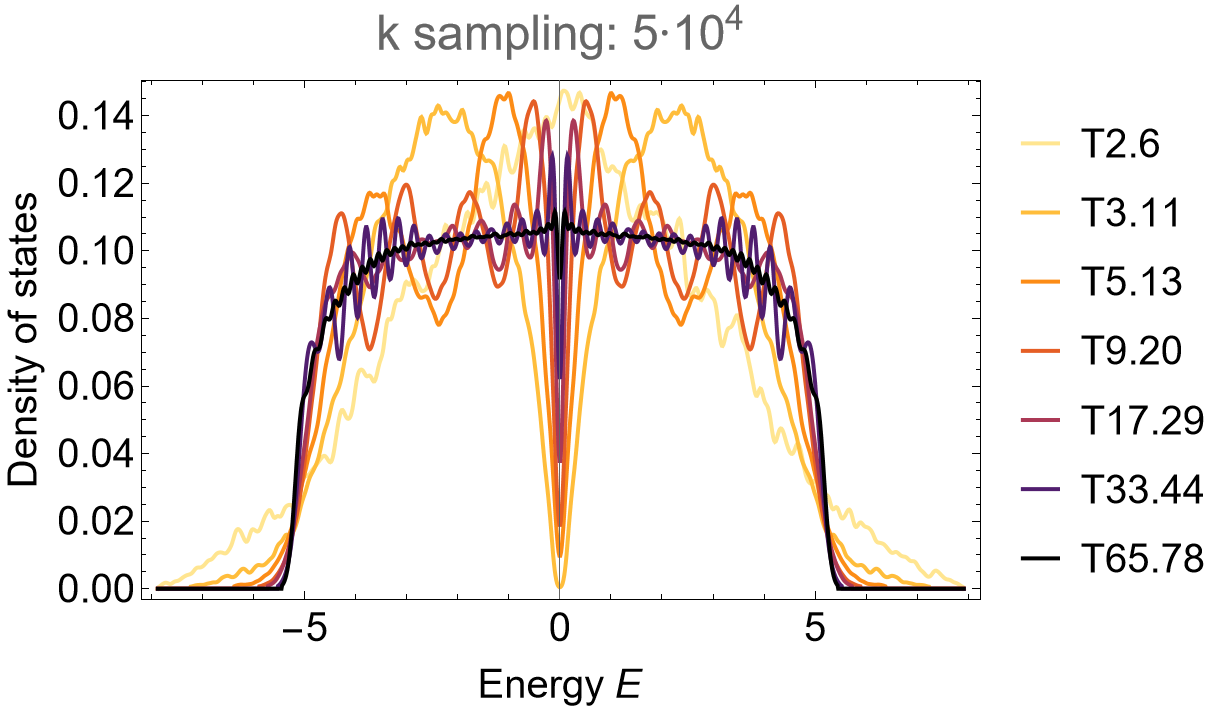
Supercell sequence 1: T2.6, T3.11, T5.13, T9.20, T17.29, T33.44 and T65.78

They are denoted as Tg.n, where g is the genus of the corresponding closed Riemann surface, i.e., the compactified unit cell, the corresponding quotients acts upon and n is the n’th quotient group with that genus. The primitive cell is identified with the quotient T2.6.

First, let us construct the proper triangle group \(\Delta^{+}\) together with the primitive cell T2.6 and the model graph, based on the tessellation graph, in GAP:

# load the HyperCells package
LoadPackage( "HyperCells" );

# set up proper triangle group
tg := ProperTriangleGroup( [ 2, 8, 8 ] );

# Primitive cell:
# ---------------

# specify the quotient defining the primitive cell
qpc := TGQuotient( [ 2, 6 ], [ 2, 8, 8 ] );

# construct symmetric primitive cell
cgpc := TGCellGraph( tg, qpc, 3 : simplify := 5 );

# elementary nearest-neighbor model
model := TessellationModelGraph( cgpc, true : simplify := 5 );
Export( model, "{8,8}-tess_T2.6_3.hcm" ); # export

The nearest-neighbor supercell model graphs for the \(\{8,8\}\)-tesselation of the hyperbolic plane are easily extracted by iterating over the list of quotients sc_lst that specify our chosen supercell sequence:

# Supercells:
# -----------

sc_lst := [[3, 11], [5, 13], [9, 20], [17, 29], [33, 44], [65, 78]];

for sc_i_index in sc_lst do
  
  # quotient group 
  qsc_i := TGQuotient( sc_i_index );

  # construct tessellation graphs
  sc_i := TGCellSymmetric(tg, qsc_i, 3);
  scmodel_i := TGSuperCellModelGraph(model, sc_i);

  # export file
  sc_i_label := StringFormatted("-tess_T2.6_3_sc-T{}.{}.hcs", sc_i_index[1], sc_i_index[2]);
  scmodel_i_name := JoinStringsWithSeparator(["{8,8}", sc_i_label], "");
  Export(scmodel_i,  scmodel_i_name);
od;

The supercell method#

We are ready to apply the supercell method in Mathematica using the HyperBloch package, provided the necessary files with the sequence of supercells are present and located in the directory of the Mathematica notebook. We load the HyperBloch package, set the working directory of the files we have created through the HyperCells package and in addition define a list of available unit cells:

<< PatrickMLenggenhager`HyperBloch`
SetDirectory[NotebookDirectory[]];
 
cells = {"T2.6", "T3.11", "T5.13", "T9.20", "T17.29", "T33.44", "T65.78"};

where we consider the unit cell T2.6 as the primitive cell. The model graph can now be imported by parsing the imported strings with the functions ImportModelGraphString:

pcmodel = ImportModelGraphString[Import["{8,8}-tess_T2.6_3.hcm"]];

We repeat this procedure for the consecutive supercell model graphs by parsing the imported strings with the function ImportSupercellModelGraphString instead:

scmodels = Association[# -> 
    ImportSupercellModelGraphString[Import["{8,8}-tess_T2.6_3_sc-" <> # <> ".hcs"]]
  &/@cells[[2 ;;]]];

In addition we extract an ordered Association, containing the genera of the compactified unit cells, programmatically:

genusLst = Join[
  Association[cells[[1]] -> pcmodel["Genus"]],
  Association[# -> scmodels[#]["Genus"] & /@ cells[[2 ;;]]] ];

Once the (supercell) model graphs are imported the corresponding Abelian Bloch Hamiltonians can be constructed. We choose to construct an elementary nearest-neighbor tight-binding model with one orbital per site, the on-site terms set to \(0\) and the nearest-neighbor hopping amplitudes set to \(-1\). Once again, we start with the primitive cell:

Hpc = AbelianBlochHamiltonian[pcmodel, 1, 0 &, -1 &, CompileFunction -> True]; 

Recall, the construction of the model on the primitive cell already defines all the model specification for the supercell. As such we just need to replace the model graph with the supercell model graphs in the first argument and pass the model graph to the option PCModel:

Hsclst = Association[# -> 
    AbelianBlochHamiltonian[scmodels[#], 1, 0 &, -1 &, PCModel -> pcmodel, CompileFunction -> True] 
  & /@ cells[[2 ;;]] ];

where we have used an Association to extract the Hamiltonians, with the previously defined labels serving as keys later. For convenience, let us collect the constructed Hamiltonians in a single Association:

Hclst = Join[Association[cells[[1]] -> Hpc], Hsclst];

Next, we want to compute the density of states. We can take advantage of the independence of different momentum sectors and parallelize the computation of the Eigenvalues, where we partition the set of Npts into Nruns subsets. This can be done as follows:

ComputeEigenvalues[cfH_, Npts_, Nruns_, genus_] :=
 Flatten@ParallelTable[
  Flatten@Table[
      Eigenvalues[cfH @@ RandomReal[{-Pi, Pi}, 2 genus]], 
    {i, 1, Round[Npts/Nruns]}], {j, 1, Nruns}, 
  Method -> "FinestGrained"]

We compute the Eigenvalues with a set of \(5 \cdot 10^4\) random samples in momentum space and \(32\) subsets:

evals =  Association[# -> ComputeEigenvalues[Hclst[#], 5 10^4, 32, genusLst[#]]&/@cells];

Let us use the following color maps for the individual unit cells:

cLst = (ColorData["SunsetColors", "ColorFunction"] /@ (1 - Range[1, 7]/7.));

We can nicely observe the convergence of the DOS:

SmoothHistogram[evals, 0.05, "PDF",
  Frame -> True, FrameLabel -> {"Energy E", "Density of states"} FrameStyle -> Black, 
  ImageSize -> 500, ImagePadding -> {{Automatic, 10}, {Automatic, 10}}, LabelStyle -> 20,
  PlotLabel -> "k sampling: 5*10^4", PlotRange -> All, PlotStyle -> cLst]

{8,8}-lattice NN-TB model DOS 1st supercell sequence

Alternative supercell sequences#

Let us also consider alternative sequences of supercells to verify the independence of the thermodynamic limit on the particular choice of sequence. We choose to construct two alternative sequences:

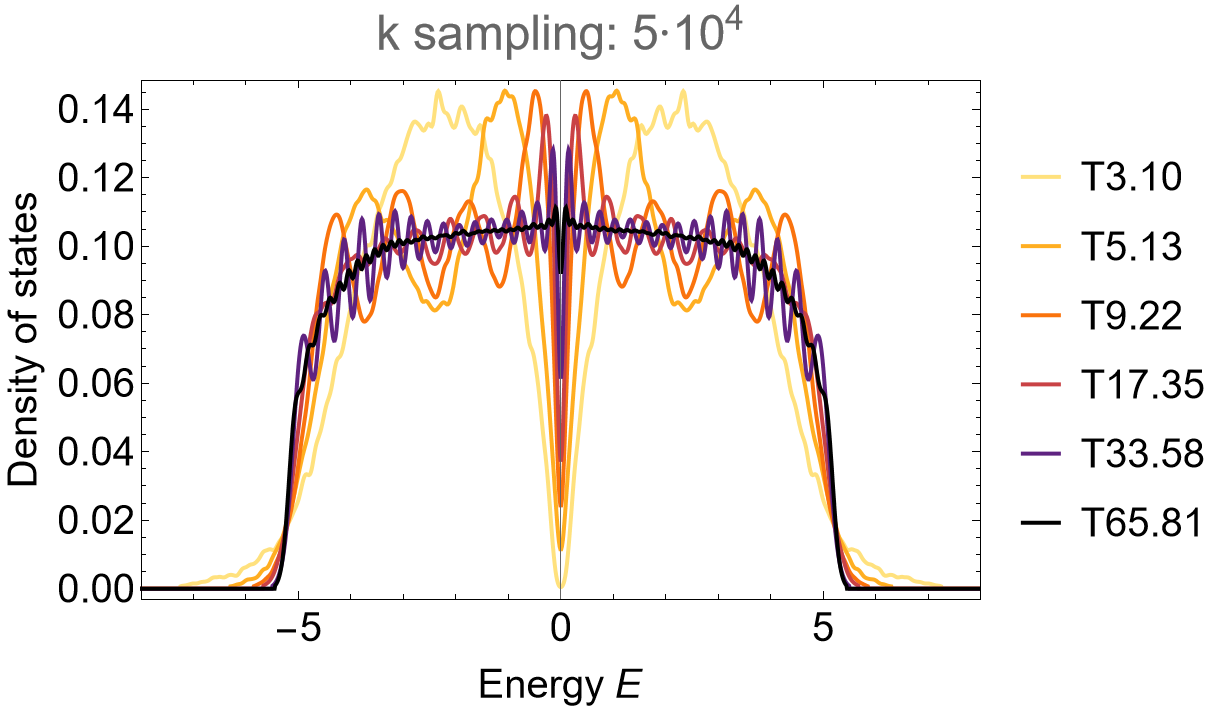
Supercell sequence 1A: T3.10, T5.13, T9.22, T17.35, T33.58 and T65.81

and

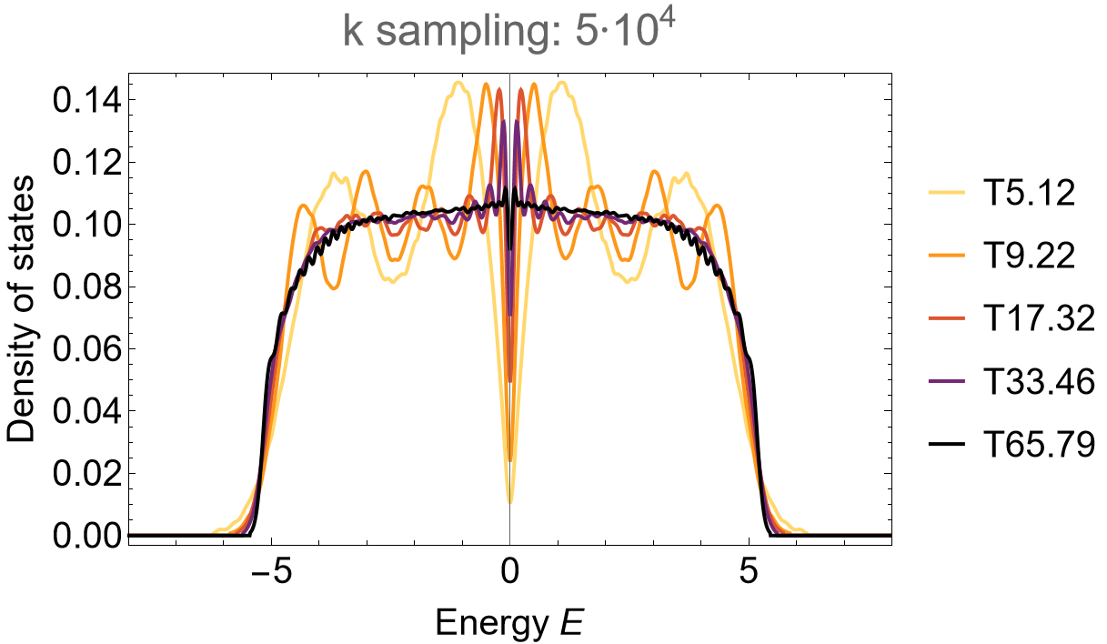
Supercell sequence 2A: T5.12, T9.22, T17.32, T33.46 and T65.79

We omit further details and leave the construction of the model and supercell model graphs in GAP, as well as the steps in Mathematica leading to the Eigenvalues for the density of states as an exercise. However, further details can be found in the downloadable files at the end of this page. The steps above can be repeated provided appropriate adjustments are preformed, resulting in the density of states as shown below. For the supercell sequence 1A the density of states looks as follows:

SmoothHistogram[evals, 0.05, "PDF",
  Frame -> True, FrameLabel -> {"Energy E", "Density of states"} FrameStyle -> Black, 
  ImageSize -> 500, ImagePadding -> {{Automatic, 10}, {Automatic, 10}}, LabelStyle -> 20,
  PlotLabel -> "k sampling: 5*10^4", PlotRange -> All, PlotStyle -> cLst]

and for the supercell sequence 2A:

SmoothHistogram[evals, 0.05, "PDF",
  Frame -> True, FrameLabel -> {"Energy E", "Density of states"} FrameStyle -> Black, 
  ImageSize -> 500, ImagePadding -> {{Automatic, 10}, {Automatic, 10}}, LabelStyle -> 20,
  PlotLabel -> "k sampling: 5*10^4", PlotRange -> All, PlotStyle -> cLst]

Download generated files Download GAP Code Download Mathematica Notebook