Haldane model#

In the previous tutorials, Supercells and Flat-bands, we have considered nearest-neighbor tight-binding models through the construction of tessellation model graphs. The HyperCells package enables the construction of extended tessellation model graphs which are comprised not only of nearest-neighbor but also next-nearest-neighbor terms. In this tutorial we will see how we can extend tessellation model graphs through the construction of next-nearest-neighbor tight-binding models on the \(\{6,4\}\)-lattice. Specifically, we will consider next-nearest-neighbor terms as small perturbations as well as a variant of the Haldane model. Additionally, we will showcase how hyperbolic lattice symmetries can be analyzed in Abelian hyperbolic band theory through the construction of point-group matrices.

Next-nearest-neighbor model graph#

Next-nearest-neighbor terms can be added through a minor modification of the usual workflow. We start by constructing the cell graph for the primitive cell in GAP:

# load the HyperCells package
LoadPackage( "HyperCells" );
tg := ProperTriangleGroup( [ 2, 4, 6 ] );

# Primitive cell:
# ---------------
qpc := TGQuotient( 1, [ 2, 4, 6 ] );
cgpc := TGCellGraph( tg, qpc, 3 : simplify := 5 );
Export( cgpc, "(2,4,6)_T2.2_3.hcc" ); # export

In order to add next-nearest-neighbor terms, a tessellation model graph needs to be specified beforehand. As such, let us construct the nearest-neighbor graph of the \(\{6,4\}\)-tesselation of the hyperbolic plane on the primitive cell:

# Construction of underlying NN-model:
# -----------------------------------
# specify underlying model graph
model := TessellationModelGraph(cgpc);

The tessellation model graph can be decorated with next-nearest-neighbor (NNN) terms through the function AddOrientedNNNEdgesToTessellationModelGraph, which introduces oriented NNN-edges with orientations in the counter-clockwise around each face based on the original tessellation model graph:

# Adding NNN terms:
# -----------------
AddOrientedNNNEdgesToTessellationModelGraph(model);
Export(model, "{6,4}-tess-NNN_T2.2_3.hcm");

We choose a supercell sequence by following the central concepts discussed in the tutorial Supercells and Coherent sequences. The model specifications are inherited by subsequent supercell model graphs:

# Supercells:
# -----------
tgQS := TGQuotientSequencesStructure(tg : boundByGenus := 10);;
sequence := LongestSequence(tgQS : quotient := 1);
sc_lst := sequence{[2..Length(sequence)]};

for sc_i_index in sc_lst do
    qsc_i := TGQuotient( sc_i_index );

    sc_i := TGCellSymmetric(tg, qsc_i, 3);
    scmodel_i := TGSuperCellModelGraph(model, sc_i);

    sc_i_label := StringFormatted("_T2.2_3_sc-T{}.{}.hcs", sc_i_index[1], sc_i_index[2]);
    scmodel_i_name := JoinStringsWithSeparator(["{6,4}-tess-NNN", sc_i_label], "");
    Export(scmodel_i,  scmodel_i_name); # export file
od;

Download generated files Download GAP Code

\(\{6,4\}\)-NNN tight-binding model:#

Before we construct the Haldane model on the \(\{6,4\}\)-lattice, let us consider a more fundamental model in order to get familiar with the procedures to assign coupling constants for next-nearest-neighbor (supercell) model graphs. As such, let us construct an elementary next-nearest-neighbor hopping model.

As usual, we load the HyperBloch package, set the working directory of the files we have created through the HyperCells package, define a list of available unit cells together with the corresponding genera of the compactified unit cells and import the cell, model and supercell model graph:

(* Preliminaries *)
<< PatrickMLenggenhager`HyperBloch`
SetDirectory[NotebookDirectory[]];

(* Labels and genera *)
cells = {"T2.2", "T5.4", "T9.3"}; 
genusLst = {2, 5, 9};

(* Import cell and model graph of the primitive cell *)
pcell = ImportCellGraphString[Import["(2,4,6)_T2.2_3.hcc"]];
pcmodel = ImportModelGraphString[Import["{6,4}-tess-NNN_T2.2_3.hcm"]];

(* Import supercell model graph *)
scmodels = Association[# -> 
  ImportSupercellModelGraphString[ 
    Import["{6,4}-tess-NNN_T2.2_3_sc-" <> # <> ".hcs"]] 
  &/@ cells[[2 ;;]]];

Let us visualize the NN and NNN-terms of the graph representation for the next-nearest-neighbor tight-binding model on the primitive cell. They are stored as directed edges, which can be extracted from the model graph as follows:

EdgeList@pcmodel["Graph"]

The first entry in the edge tags (the nested list above the arrow) indicate the if the edge connects NN-vertices or NNN-vertices, indicated with integers 1 and 2, respectively. We have already discussed the edges that connect NN-vertices in Getting started with the HyperBloch package. Now, for the NNN-edges the remaining edge tags are of the form {f, e1, e2}, f is the position of the face characterizing the edge in the list of faces in the model graph, and e1, e2 are the positions of the nearest-neighbor edges that together connect the same vertices as the next-nearest-neighbor edge in the list of edges in the model graph.

We can visualize the corresponding edges by using the option EdgeFilter of the function ShowCellGraphFlattened. This enables us to visualize edges connecting NN-vertices or NNN-vertices separately:

Row[
 Table[
  Module[{filterFunction},
   filterFunction[edge_, j_] := If[j < 3, edge[[3, 1]] == j, edge[[3, 1]] < j];
   VisualizeModelGraph[pcmodel, 
      CellGraph -> pcell, 
      Elements -> <|
        ShowCellBoundary -> {ShowEdgeIdentification -> True},
        ShowCellGraphFlattened -> {EdgeFilter -> (filterFunction[#, j] &)}
      |>,
      ImageSize -> 300, NumberOfGenerations -> 3]],
  {j, 3}]]

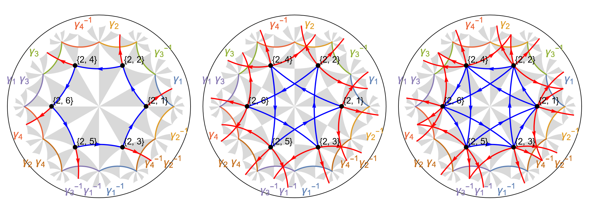
In order to construct the Abelian Bloch Hamiltonian let us recall the general startegy to endow the model graphs with coupling constants, see Getting started with the HyperBloch package. The list of edges, accessed through calling EdgeList@pcmodel["Graph"], allows us to associate distinct hopping amplitudes h1 and h2 with the NN and NNN-terms, respectively. It contains 12 directed edges connecting NN-vertices followed by 24 directed edges connecting NNN-vertices, thus:

(* NN-terms *)
nnVec = ConstantArray[h1, 12];

(* NNN-terms *)
nnnVec = ConstantArray[h2 , 24];

The hopping amplitudes can be assigned through an Association, with edges as keys and hopping amplitudes as values:

(* Construct association *)
hoppingVec = Join[nnVec, nnnVec];
hoppingsPC = AssociationThread[EdgeList@pcmodel["Graph"] -> hoppingVec];

The corresponding Hamiltonians are given by:

(* Hamiltonian for the primitive cell *)
Hpc = AbelianBlochHamiltonian[pcmodel, 1, 0 &, hoppingsPC, CompileFunction -> True];

(* Hamiltonians for the supercells *)
Hsclst = Association[# -> 
    AbelianBlochHamiltonian[scmodels[#], 1, 0 &, hoppingsPC, PCModel -> pcmodel, CompileFunction -> True] 
  &/@ cells[[2 ;;]]];

(* All *)
Hclst = Join[Association[cells[[1]] -> Hpc], Hsclst];

As usual, we compute the density of states of this sequence of supercells by random samples in the Brioullin zone, where we use the function ComputeEigenvalues, which can be found in the dropdown menu Needed function above. We choose to treat the next-nearest-neighbor contributions as a weak coupling between sites, as such we set h1 to \(1\) and h2 to \(0.05\):

(* Eigenvalues *)
evals = Association[# -> ComputeEigenvalues[Hclst[#] /. {h1 -> 1, h2 -> 0.05}, 10^4, 32, genusLst[#]]&/@cells];

(* Color maps *)
cLst = (ColorData["SunsetColors", "ColorFunction"] /@ (1 - Range[1, 3]/3.));

(* Visualize *)
SmoothHistogram[evals, 0.01, "PDF",
  Frame -> True, FrameLabel -> {"Energy E", "Density of states"} FrameStyle -> Black, 
  ImageSize -> 500, ImagePadding -> {{Automatic, 10}, {Automatic, 10}}, LabelStyle -> 20,
  PlotLabel -> "k sampling: 10^4", PlotRange -> All, PlotStyle -> cLst]

Haldane model#

The next-nearest-neighbor tight-binding model can easily be extended to a variant of the Haldane model. Analogous to original Haldane model, our variant should thread the \(\{6,4\}\)-lattice by local magnetic fluxes with net zero flux per hyperbolic hexagon. Let us highlight the central hyperbolic hexagon, which should be threaded with a net zero flux. The hexagon is associated with a face in the model graph and can be extracted through the function GetCellGraphFace:

face = GetCellGraphFace[pcmodel, pcmodel["Faces"][[1]]];

The returned object is a Polygon that can be visualized in the Poincaré disk as follows:

Show[
 VisualizeModelGraph[pcmodel,
  CellGraph -> pcell,
  Elements -> <|
    	ShowCellGraphFlattened -> {},
    	ShowCellBoundary -> {ShowEdgeIdentification -> True}
    |>,
  ImageSize -> 300,
  NumberOfGenerations -> 3],
 
 Graphics[{Opacity[0], FaceForm[{Darker@Green, Opacity[0.5]}], face}]
]

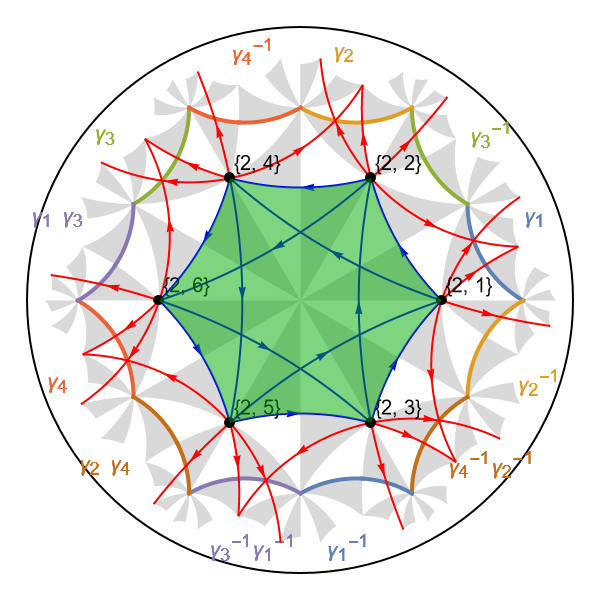
The directed edges for the NNN-terms are oriented such that a Peierls substitution can be performed by multiplying the previously defined constant vector nnnVec by a phase \(e^{i\phi}\) . The resulting \(\{6,4\}\)-lattice is threaded by local magnetic fluxes with net zero flux per hyperbolic hexagon:

(* NNN-terms *)
phase = Exp[I Phi];
nnnVec = phase * nnnVec;

(* Construct association *)
hoppingVec = Join[nnVec, nnnVec];
hoppingsPC = AssociationThread[EdgeList@pcmodel["Graph"] -> hoppingVec];

Since the hyperbolic hexagons have an even number of sides the lattice can be considered as bipartite such that a sublattice mass can be realized by a staggered on-site potential \(\pm m\). It is instructive to take a look at the list of vertices in the model graph:

VertexList@pcmodel["Graph"]

Vertices tessellation model {6,4}-lattice

Comparing the list of vertices with the model representation we have previously visualized, we can assign the staggered on-site potential as follows:

mVec = m {1, -1, -1, 1, 1, -1};
onsitePC = AssociationThread[VertexList@pcmodel["Graph"] -> mVec];

The Abelian Bloch Hamiltonians are given by:

(* Hamiltonian for the primitive cell *)
Hpc = AbelianBlochHamiltonian[pcmodel, 1, onsitePC, hoppingsPC, CompileFunction -> True];

(* Hamiltonians for the supercells *)
Hsclst = Association[# -> 
    AbelianBlochHamiltonian[scmodels[#], 1, onsitePC, hoppingsPC, PCModel -> pcmodel, CompileFunction -> True] 
  &/@ cells[[2 ;;]]];

(* All *)
Hclst = Join[Association[cells[[1]] -> Hpc], Hsclst];

The density of states can be computed as usual:

(* Eigenvalues *)
evals = Association[# -> 
    ComputeEigenvalues[Hclst[#] /. {h1 -> 1, h2 -> 0.5, m -> 0, Phi -> Pi/2}, 10^4, 32, genusLst[#]]
  &/@cells];

(* Visualize *)
SmoothHistogram[evals, 0.01, "PDF",
  Frame -> True, FrameLabel -> {"Energy E", "Density of states"} FrameStyle -> Black, 
  ImageSize -> 500, ImagePadding -> {{Automatic, 10}, {Automatic, 10}}, LabelStyle -> 20,
  PlotLabel -> "k sampling: 10^4", PlotRange -> All, PlotStyle -> cLst]

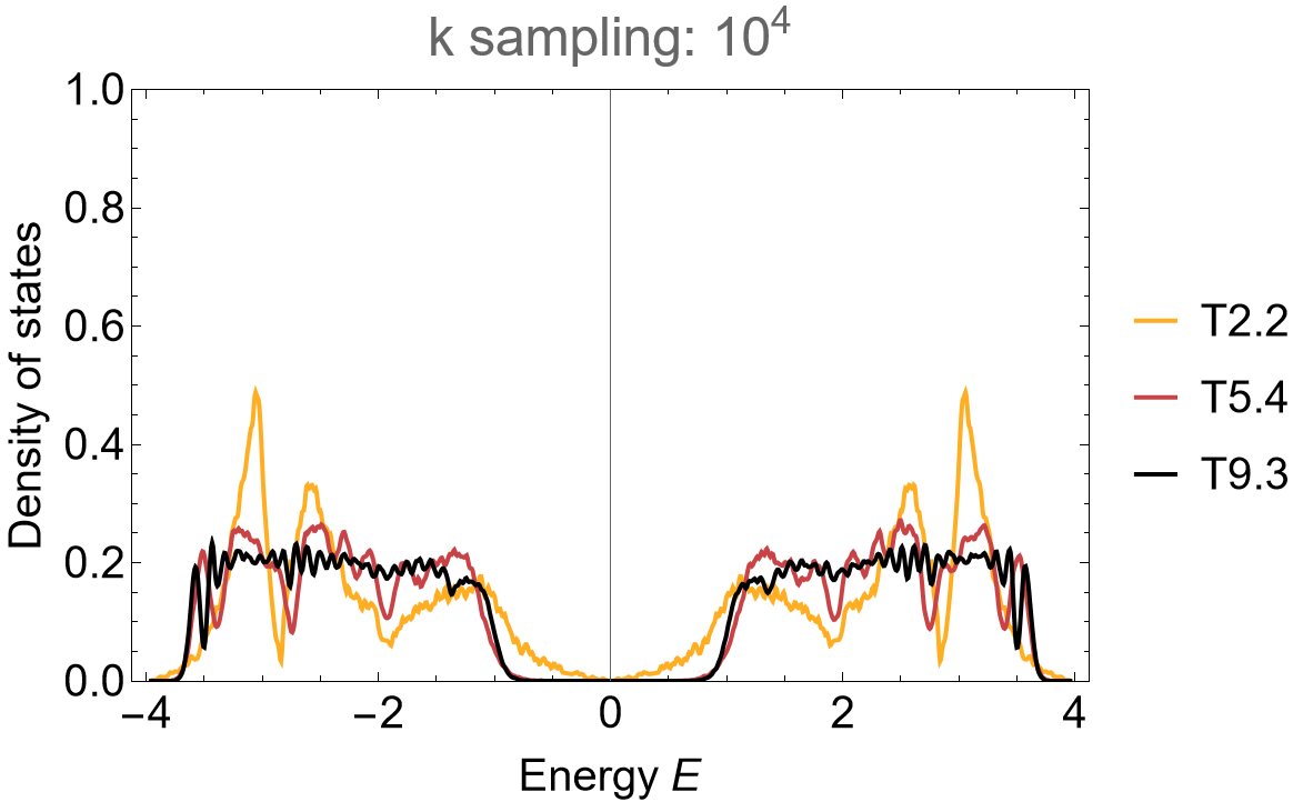
The application of the supercell method reveals spurious feature in the density of states of the primitive cell when using the Abelian Hyperbolic band theory. Some of the Abelian states lie outside the energy range with finite density in the thermodynamic limit and thus the band touching at zero energy can be considered a finite size effect.

Download Mathematica Notebook

Point-group matrices#

Symmetry elements of triangle groups might act non-trivially on hyperbolic momenta. As such, the degrees of freedom of observables and topological invariants, like the first Chern numbers in momentum space, might be constrained by the hyperbolic lattice symmetries of underlying models. We can determine how hyperbolic momenta transform as hyperbolic lattice symmetry transformations act on Abelian states. This can be extracted by constructing point-group matrices.

Point-group matrices can be constructed by specifying the hyperbolic lattice symmetries in terms of generators of the triangle group \(\Delta(2,q,p)\) or the proper triangle group \(\Delta^{+}(2,q,p)\). Let us visualize the action of the symmetry generators on the fundamental Schwarz triangle s_f of the \(\{6,4\}\)-tesselation of the hyperbolic plane:

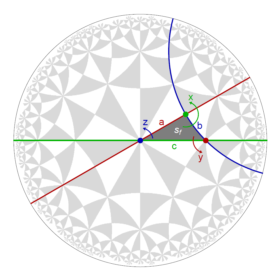
For example, the generator z of the proper triangle group \(\Delta^{+}\) is a composition of two reflection generators c*a of \(\Delta\). The fundamental Schwarz triangle is rotated by \(2 \pi/6\) in counter clockwise direction to an adjacent copy under the action of the operator z. We can construct the operator as follows:

# proper triangle group 
D := FpGroup(tg);

# symmetry
z := D.3;
symmetry := z;
symName := "z";

Point-group matrices define representations of point groups \(G^{(m)}\cong\Delta/\Gamma^{(m)}\). This implies that it is sufficient to construct the point-group matrices for a minimal set of operators, such that matrix multiplications can be performed in order to construct the point-group matrices of other elements in the point group. As such, we first need to construct the point-group matrices for the rotation generators of the triangle group group for any given unit cell identified through a corresponding triangle group quotient \(\Delta/\Gamma^{(m)}\).

They can be computed through the function PGMatricesOfGenerators, which takes the triangle group, proper triangle group and a triangle group quotient as arguments. As such, we first need to construct the triangle group:

# TriangleGroup obj.
fulltg := TriangleGroup( [ 2, 4, 6 ] );

Next, let us construct the point-group matrices of the triangle generators for the primitive cell:

# get the PGMatricesOfGenerators
pgMatGs := PGMatricesOfGenerators(fulltg, tg, qpc);

The point-group matrix for the symmetry z can now be evaluated through the function EvaluatePGMatrix:

gap>  EvaluatePGMatrix(z, pgMatGs);
[ [  0, -1,  0,  0 ], 
  [  0,  0, -1,  0 ], 
  [  0,  1,  0, -1 ], 
  [  1,  0,  0,  0 ] ]

Let us construct a particular point-group matrix for a symmetry analysis \(\{6,4\}\)-Haldane model. In principle, there are two sets of symmetry operations that leave the model invariant, which are dictated by the configuration of the coupling constants, i.e, if the staggered on-site potential is non-zero or not. However, we will focus on a particular symmetry transformation that is common among them.

The model is left invariant under a reflection c composed with time reversal T (note that an anti-unitary symmetry transformation, like time reversal, leads to an overall sign change of the point-group matrix, which we will consider later).

We have already constructed the corresponding point-group matrix through the function PGMatricesOfGenerators. However, let us choose to construct it once more as a sparse representation by passing the option sparse:

# get the PGMatricesOfGenerators
pgMatGs := PGMatricesOfGenerators(fulltg, tg, qpc : sparse := true);

A set of point-group matrices can only be exported by first calling the function PGMatrices. We choose to export the point-group matrices for c and z. However, we only need to specify the z, since the point-group matrices of the triangle group generators will be inherited:

# construct and export the PGMatrices
pgMat_T2_2 := PGMatrices(symmetry, pgMatGs : symNames := symName);
Export(pgMat_T2_2, "(2,4,6)-T2.2-pgMat_z_sparse.hcpgm");

We can repeat the procedure for the chosen supercell sequence:

# Quotients T5.4, T9.3 (supercells):
# ---------------------------------
for sc_i_index in sc_lst do
  qsc_i := TGQuotient( sc_i_index );

  # get the PGMatricesOfGenerators
  pgMatGs := PGMatricesOfGenerators(fulltg, tg, qsc_i : sparse := true);

  # construct and export the PGMatrices
  pgMat_sc_i := PGMatrices(symmetry, pgMatGs : symNames := symName);

  sc_i_label := StringFormatted("(2,4,6)-T{}.{}-pgMat_z_sparse.hcpgm", sc_i_index[1], sc_i_index[2]);
  Export(pgMat_sc_i, sc_i_label);
od;

Download generated files Download GAP Code

Application#

Point-group matrices can be used to conduct symmetry analysis on any given (supercell) model graph. Let us perform a symmetry transformation for the variant of the Haldane model we have considered above, in order to see how the corresponding spectra are effected.

The point-group matrices can be imported analogously to (supercell) model graphs. As such, the Import function is used to read the file, while the ImportPGMatricesString function is used to parse the string and construct the point-group matrices:

pgMatSc = Association[# -> ImportPGMatricesString[Import["(2,4,6)-" <> # <> "-pgMat_z_sparse.hcpgm"]]&/@cells];

The spectrum of the Haldane model should be left invariant under the hyperbolic lattice symmetry transformation c. This can easily be verified by an explicit transformation of the hyperbolic momenta through the following modification of the function defined in the dropdown menu Needed function above:

ComputeEigenvalues[cfH_, pgMat_, Npts_, Nruns_, genus_] :=
 Flatten@ParallelTable[
   Flatten@Table[
     Eigenvalues[cfH @@ (Dot[-pgMat,RandomReal[{-Pi, Pi}, 2 genus]])], 
     {i, 1, Round[Npts/Nruns]}],
   {j, 1, Nruns}, Method -> "FinestGrained"]

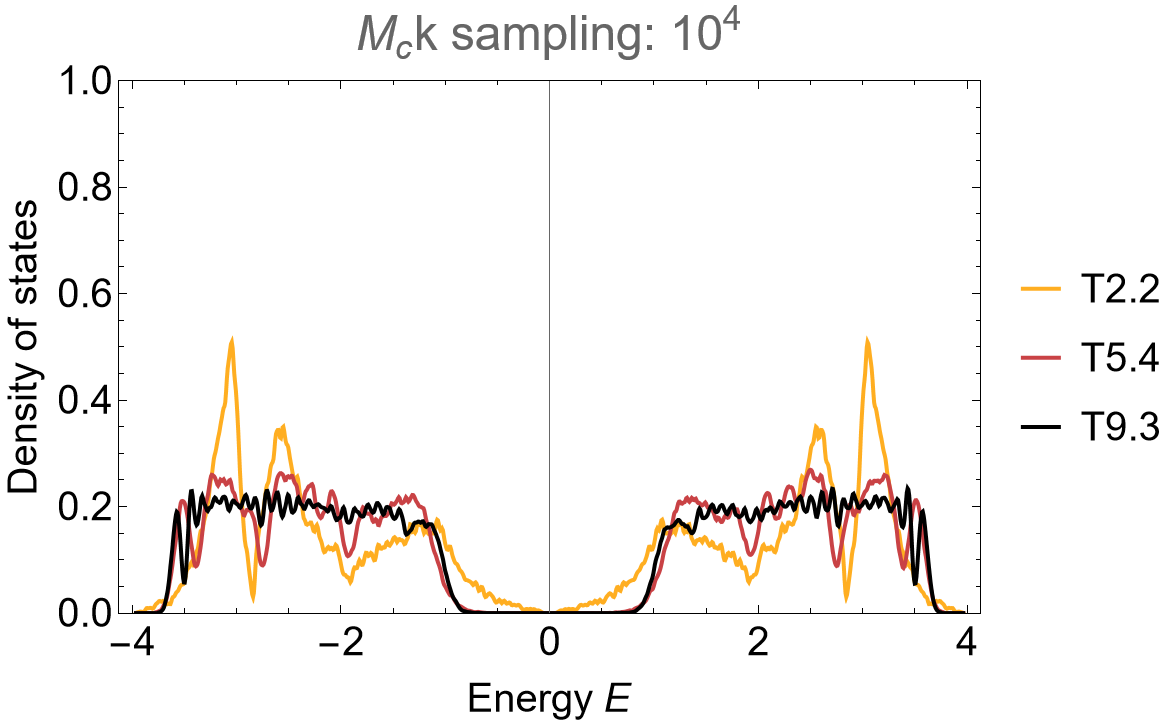
where we have multiplied the point-group matrix pgMat by -1 in order to account for the anti-unitarity of the transformation. The point-group matrices can be extracted by using the corresponding symmetry names as keys. We compute the Eigenvalues with a set of \(10^4\) random samples in momentum space, partitioned into \(32\) subsets as before and pass the point-group matrix for the symmetry transformation cT to the function:

evals = Association[# -> 
  ComputeEigenvalues[Hclst[#] /. {h1 -> 1, h2 -> 0.5, m -> 0, Phi -> Pi/2}, 
    -pgMatSc[#]["c"], 10^4, 32, genusLst[#]] 
  & /@ cells];

The resulting density of states is unchanged (aside from negligible changes due to random sampling in combination with a relatively small sample size):

SmoothHistogram[evals, 0.01, "PDF",
  Frame -> True, FrameLabel -> {"Energy E", "Density of states"} FrameStyle -> Black, 
  ImageSize -> 500, ImagePadding -> {{Automatic, 10}, {Automatic, 10}}, LabelStyle -> 20,
  PlotLabel -> "Mc k sampling: 10^4", PlotRange -> All, PlotStyle -> cLst]

Download Mathematica Notebook

Visualize reflections and rotations (bonus):#

The visualization toolbox of the HyperBloch package enables us to visualize how symmetries act on the graph representation of models. Let us reproduce the illustration of how generators of the triangle group and proper triangle group act on the fundamental Schwarz triangle.

Fundamental Schwarz triangle#

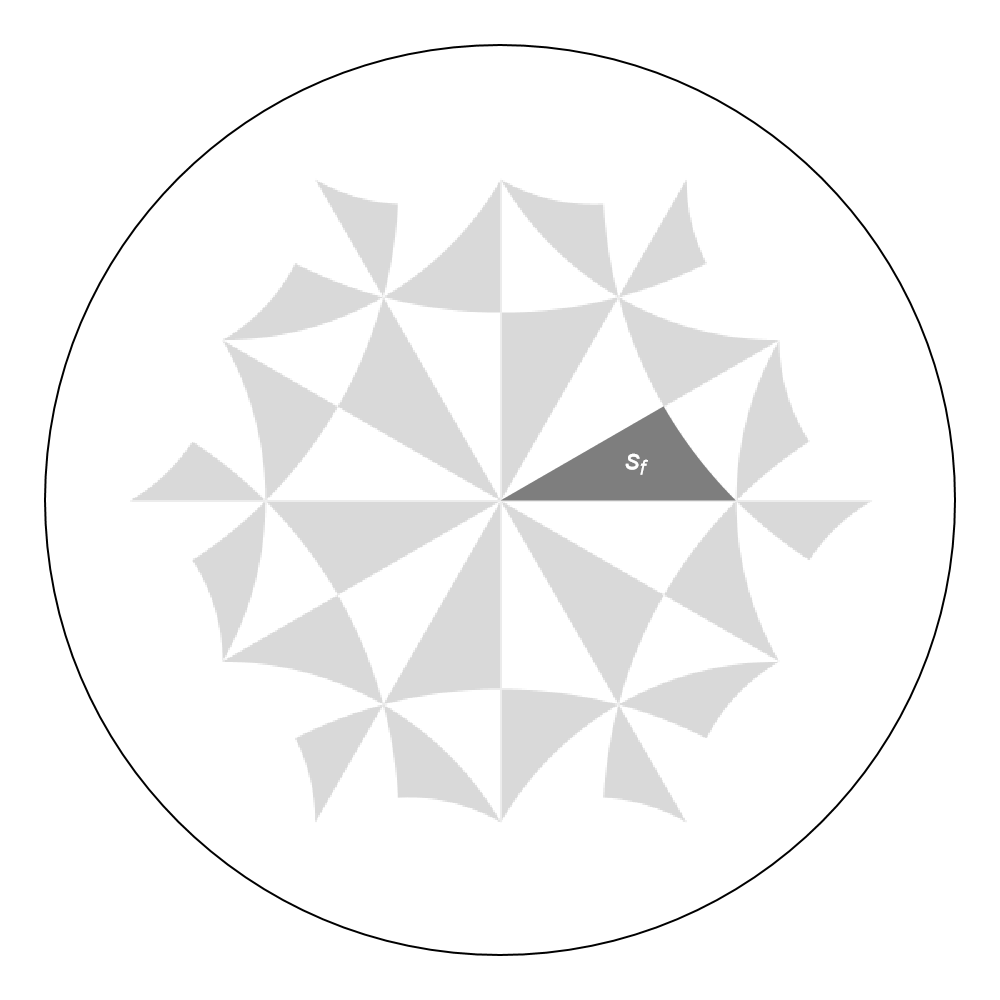
We can highlighted individual Schwarz triangles in the Poincaré disk through the function GetSchwarzTriangle. For example, let us extract the Polygon representing the fundamental Schwarz triangle associated with the identity element in the proper triangle group \(\Delta^+(2,4,6)\):

sf = GetSchwarzTriangle[{2, 4, 6}, "1"];

The fundamental Schwarz triangle can be visualized in the Poincaré disk, we may choose the function ShowTriangles to achieve this:

g1 = Show[
  ShowTriangles[{2, 4, 6}, ImageSize -> 300, NumberOfGenerations -> 2],
  Graphics[{Darker[Gray, 0.01], sf}],
  Graphics[{Text[Style["s_f", 15, Thick, White], {0.3, 0.09}]}],
  
  ImageSize -> 500
]

Reflections#

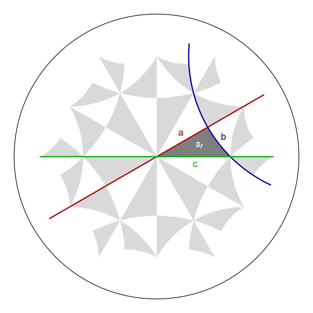
The reflections associated with the triangle group generators acting on the fundamental Schwarz triangle \(s_{f}\) can be indicated in the Poincaré disk through the function GetEdge which enables us to extract a Line representing the edge (or succession of edges) specified by vertices. We choose pairs of vertices such that each line extends a side of \(s_{f}\) shown as hyperbolic geodesics. Each vertex is of the form \(\{w_{i},\) “\(g_{i}\)” \(\}\) , where \(w_{i}\) specifies a Wyckoff position and “\(g_{i}\)” a symmetry operation:

aLine = GetEdge[{2, 4, 6}, {{1, "z^3*x"}, {1, "z^3*x*z^3"}}];
bLine = GetEdge[{2, 4, 6}, {{2, "x*y^2"}, {2, "x*y^2*x"}}];
cLine = GetEdge[{2, 4, 6}, {{3, "y^2"}, {3, "y^2*z^3"}}];

The lines can be visualized in Poincaré disk together with the fundamental Schwarz triangle as follows:

Show[g1,
  
  Graphics[{Darker[Red, 0.3], AbsoluteThickness[2], aLine}],
  Graphics[{Darker[Blue, 0.3], AbsoluteThickness[2], bLine}],
  Graphics[{Darker[Green, 0.3], AbsoluteThickness[2], cLine}],
  
  Graphics[{Darker[Red, 0.3], Text[Style["a", 15, Thick], {0.17, 0.17}]}],
  Graphics[{Darker[Blue, 0.3], Text[Style["b", 15, Thick], {0.47, 0.14}]}],
  Graphics[{Darker[Green, 0.3], Text[Style["c", 15, Thick], {0.27, -0.05}]}],
  
  ImageSize -> 500
]

Rotations#

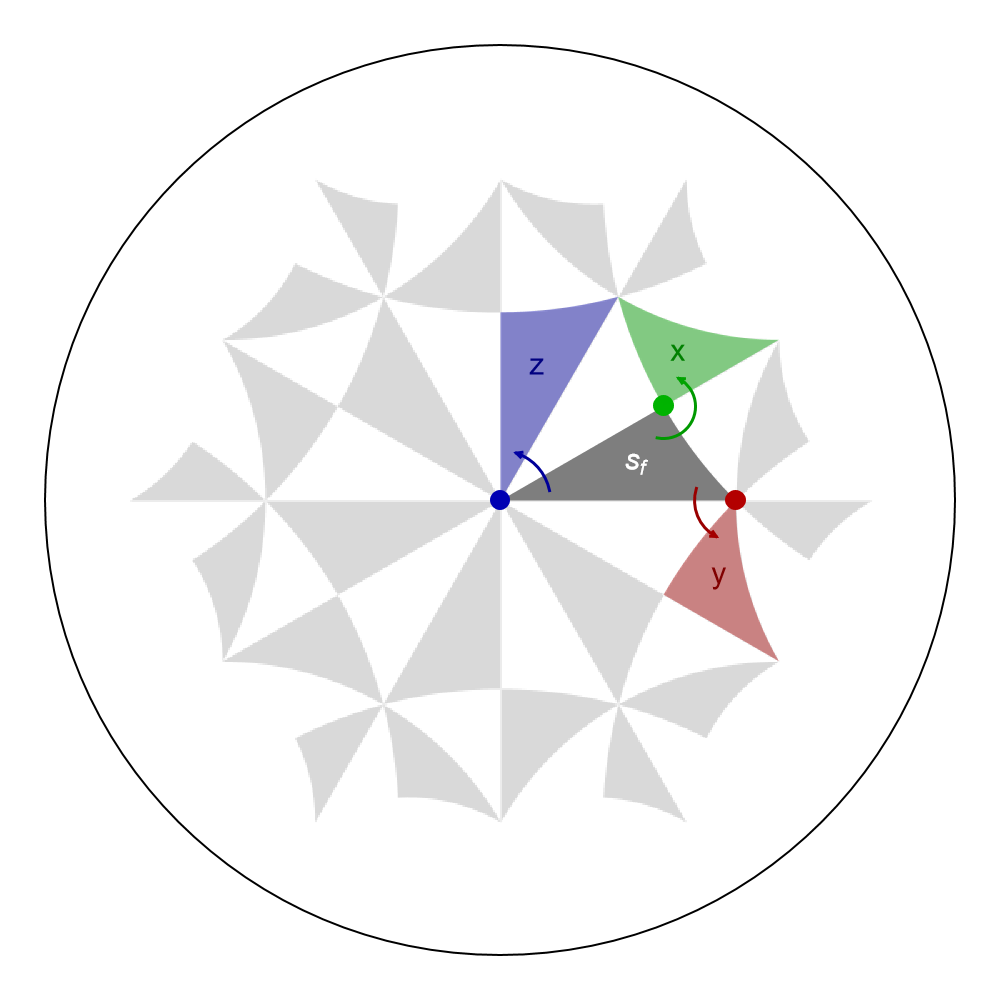
Similarly, the rotations associated with the proper triangle group generators acting on the fundamental Schwarz triangle \(s_{f}\) can be indicated in the Poincaré disk through the functions GetSchwarzTriangle and GetVertex, the latter enables us to extract a Point representing a vertex in the Poincaré disk. Under the right action of the proper triangle group generators the fundamental Schwarz triangle is transported as follows:

xsf = GetSchwarzTriangle[{2, 4, 6}, "x"];
ysf = GetSchwarzTriangle[{2, 4, 6}, "y"];
zsf = GetSchwarzTriangle[{2, 4, 6}, "z"];

The Points representing the vertices of the fundamental Schwarz triangle, which are of the form \(\{w_{i},\) “\(g_{i}\)” \(\}\), can be extracted as follows:

x = GetVertex[{2, 4, 6}, {1, "1"}];
y = GetVertex[{2, 4, 6}, {2, "1"}];
z = GetVertex[{2, 4, 6}, {3, "1"}];

In addition, let us indicate the rotations with segments of circles:

arcArrow[a_, r_, {start_, end_}] := Module[{arrForm},
  arrForm = Graphics[Line[{{{-1, 1/2}, {0, 0}, {-1, -1/2}}}]];
  {Arrowheads[{{.005, 1, arrForm}}], Arrow[Circle[a, r, {start, end}]]}
]

xar = arcArrow[x[[1]], 0.07, {3 Pi/2 - 0.2, 5 Pi/2 - 0.5}];
yar = arcArrow[y[[1]], 0.09, {Pi - 0.3, 3 Pi/2 - 0.5}];
zar = arcArrow[z[[1]], 0.11, {0.2, Pi/3 + 0.2}];

The vertices and Schwarz triangles can be visualized in Poincaré disk together with the fundamental Schwarz triangle as follows:

Show[g1,
 
 Graphics[{Darker[Green, 0.3], PointSize[0.02], x}],
 Graphics[{Darker[Red, 0.3], PointSize[0.02], y}],
 Graphics[{Darker[Blue, 0.3], PointSize[0.02], z}],
 
 Graphics[{Darker[Green, 0.4], AbsoluteThickness[1.5], xar}],
 Graphics[{Darker[Red, 0.4], AbsoluteThickness[1.5], yar}],
 Graphics[{Darker[Blue, 0.4], AbsoluteThickness[1.5], zar}],
 
 Graphics[{Darker[Green, 0.3], Opacity[0.4], xsf}],
 Graphics[{Darker[Red, 0.3], Opacity[0.4], ysf}],
 Graphics[{Darker[Blue, 0.3], Opacity[0.4], zsf}],
 
 Graphics[{Darker[Green, 0.5], Text[Style["x", 15, Thick], {0.39, 0.33}]}],
 Graphics[{Darker[Red, 0.5], Text[Style["y", 15, Thick], {0.48, -0.16}]}],
 Graphics[{Darker[Blue, 0.5], Text[Style["z", 15, Thick], {0.08, 0.3}]}],
 
 ImageSize -> 500
]

Alternatively, we may as well use the function ShowCellSchwarzTriangles together with the option TriangleRange and ShowTriangleLabels if the Schwarz triangles are within the unit cell specified by the (supercell) model graph, in order to indicate the Schwarz triangles, instead of the function GetSchwarzTriangle,:

Show[g1,
 ShowCellSchwarzTriangles[pcmodel,
  ShowTriangleLabels -> True,
  TriangleLabelStyle -> Directive[Black, Italic, 18],
  TriangleStyle -> Lighter[Gray, 0.15],
  TriangleRange -> {1, 2, 7, 12}],
 
 Graphics[{Darker[Green, 0.3], PointSize[0.02], x}],
 Graphics[{Darker[Red, 0.3], PointSize[0.02], y}],
 Graphics[{Darker[Blue, 0.2], PointSize[0.02], z}],
 
 Graphics[{Darker[Green, 0.4], AbsoluteThickness[3], xar}],
 Graphics[{Darker[Red, 0.4], AbsoluteThickness[3], yar}],
 Graphics[{Darker[Blue, 0.3], AbsoluteThickness[3], zar}],
 
 Graphics[{Darker[Green, 0.4], Text[Style["x", 20, Thick], {0.48, 0.20}]}],
 Graphics[{Darker[Red, 0.4], Text[Style["y", 20, Thick], {0.38, -0.06}]}],
 Graphics[{Darker[Blue, 0.4], Text[Style["z", 20, Thick], {0.12, 0.12}]}],
 
 ImageSize -> 500
 ]

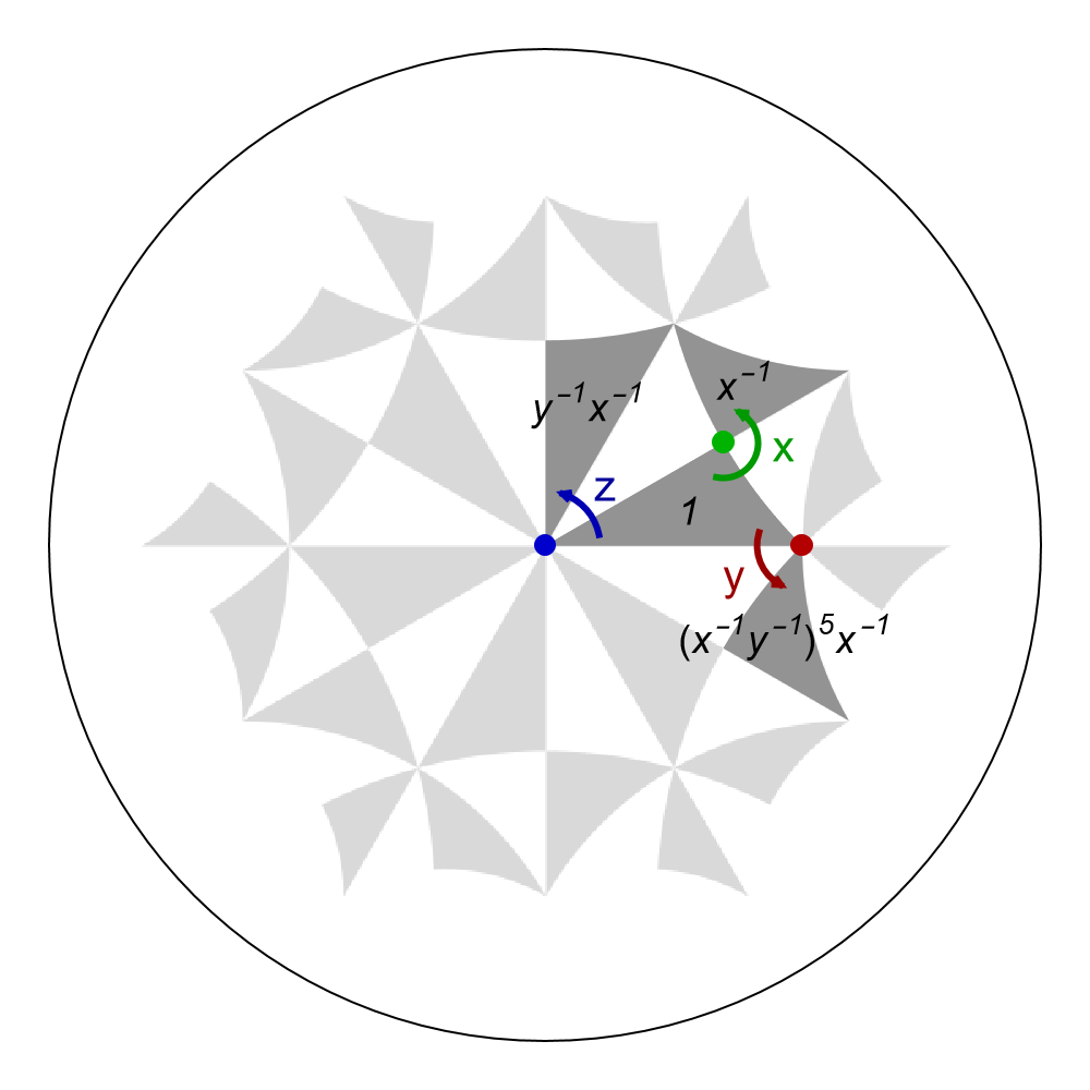
The triangles are labeled by the corresponding right action of the elements in \(T_{\Delta}(\Gamma)\) acting on the fundamental Schwarz triangle \(s_f\), written as words in terms of the generators \(x, y, z\) of the proper triangle group \(\Delta^{+}\). These labels are equivalent to the colored labels we have added manually.